
Introduction
These notes assume a basic understanding of budget lines and indifference curves. One place to go online for this information is https://en.wikipedia.org/wiki/Indifference_curve. What follows is calculus-free. At times this means that the discussion gets a little tedious but hang in there or skip ahead.
The Slope of the Indifference Curve
Think about Fred’s indifference curve. The slope of Fred’s indifference curve is the value to Fred of a little more hamburger, measured in terms of french fries. The slope is how much Fred is willing to pay to get a little bit more hamburger. Instead of being measured in money, it is measured in french fries. We will be comparing value and cost and because the true cost of a hamburger to Fred is the french fries he must give up, it is useful to measure the value of a hamburger in french fries also.
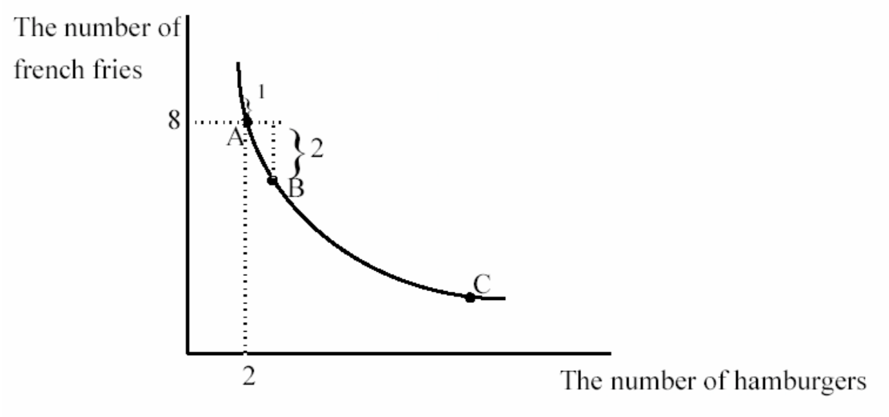
The figure shows Fred’s indifference curve through point A, the combination of 8 french fries and 2 hamburgers. How much is Fred willing to pay for a third hamburger? The answer is two french fries. He would like to pay less. But if he gets a third hamburger, he is willing to pay up to 2 french fries because he will be indifferent if he does so. The value to Fred of a third hamburger depends on how many french fries he already is consuming. The answer might not be the same if he had only two french fries. It is unlikely that he would be willing to pay two french fries to get a third hamburger in that situation.
The value to Fred of a 3rd hamburger given that Fred is consuming at point A is 2 french fries. The slope of the indifference curve at A is very close to being equal to this value of 2. To see this look at the slope of the line between A and B. The slope is the vertical distance separating the two points, divided by the horizontal distance, the rise- over-the-run. The absolute value of the slope is 2–the actual value to Fred of one more hamburger given that he is at A. But the slope of the indifference curve at A is very close to the slope of the line connecting A and B.
The indifference curve does not have a single slope because it is not a straight line. The slope of a curve must be defined as the slope at a particular point. Take point A for example. The slope of the indifference curve at A is the slope of the line tangent to point A–the line that just kisses the indifference curve at A. This is shown in the figure as the dotted line touching A. Notice that the slope of the dotted line is almost the same as the slope of the line connecting A and B, which told us the value of an extra hamburger. So the slope of an indifference curve is a pretty good measure of how much someone is willing to pay to get one more hamburger.
To see that this interpretation of the slope of an indifference curve makes sense, consider a point like C. At C, Fred has a lot of hamburgers relative to french fries, so it would make sense if his value of an extra hamburger given that he is at C would be less than the value of an extra hamburger at A. And indeed, the slope of the indifference curve at C is low, a number like 1/3. Fred would be willing to give up only 1/3 of a french fry to get one more hamburger if he is consuming the bundle at C.
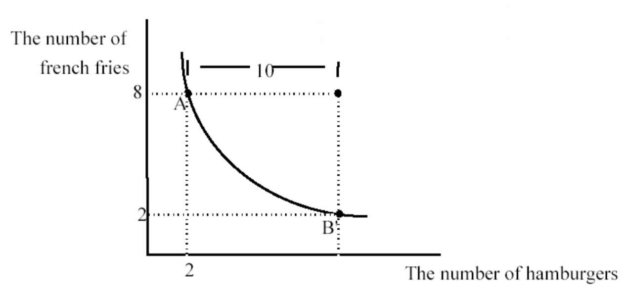
The slope at A is actually a little bit greater than the slope of the line connecting A and B–the latter being the value of one whole extra hamburger. The value of one whole extra hamburger given that Fred is at A is 2 french fries. The slope of the line tangent at A might be something like 2.05. They are very close. Why are they different? The slope at A is the value of just a little more hamburger–the slope of the line connecting A and B is the value of an entire extra hamburger. For example, the slope of the indifference curve at A is not a good approximation for how much Fred would be willing to pay for 10 more hamburgers. If we used the measure of 2.05, we would predict that Fred would be willing to pay 20.5 french fries to get 10 more hamburgers. But this would put Fred on a much lower indifference curve. It doesn’t even make sense–he only has 8 french fries to give up. The correct number of french fries Fred is willing to pay to get 10 more hamburgers is in fact, 6:
 So the slope of the indifference curve is only a good approximation of willingness to pay, or value, when considering a small increase in the number of hamburgers. The slope is a better and better approximation as we consider smaller and smaller amounts of extra hamburger. The intuition for this result is that Fred is willing to pay 2 french fries to get another hamburger when he has 8 french fries and two hamburgers. If he made the exchange to the point three hamburgers, 6 french fries, his willingness to pay for an extra hamburger is going to change because he now has a different combination of hamburgers and french fries. If it didn’t change, his indifference curve would be a straight line. We use the slope at A to approximate the value of one more hamburger. As long as one more hamburger is a “small” amount, the slope at A is a good approximation of the value Fred places on getting a little more hamburger.
To see the point, suppose a hamburger can be divided up into 10 bites. The first bite past two hamburgers, given that Fred also has 8 french fries might be worth just a little bit less than .205 french fries (or a bit more than 1/5th of a french fry). (Do you see where the number .205 comes from?). But the next bite is going to be worth a little bit less than that because now Fred has a little more hamburger (1/10) and a smaller number (about 1/5th less) of french fries. As a result, Fred’s willingness to pay for the second bite of the third hamburger will be a little less than .205. So the total value of the entire third hamburger will be less than 10 x .205 or less than 2.05. In fact, it is equal to 2, the slope of the line connecting A and B. But the slope of the indifference curve at A is close to the value of the third hamburger, when I have 2 hamburgers and 8 french fries.
Conclusion: We would like to know how many french fries Fred is willing to give up to get more hamburger. But how much more hamburger are we talking about? We could measure the value of a particular increase in hamburger consumption by connecting points like A and B. Instead, it will be sufficient to measure Fred’s value of a little bit more hamburger, which is closely approximated by the slope of the indifference curve at each point in H, F space. At every possible combination of H and F, Fred has a willingness to pay for a little more hamburger which is measured by the slope of his indifference curve.
REMEMBER: THE SLOPE OF THE INDIFFERENCE CURVE AT ANY POINT IS FRED’S WILLINGNESS TO PAY FOR A LITTLE MORE HAMBURGER. IT IS HOW MANY FRENCH FRIES FRED IS WILLING TO GIVE UP TO GET A LITTLE MORE HAMBURGER.
A GOOD EXERCISE TO SEE IF YOU UNDERSTAND INDIFFERENCE CURVES: COULD THE INDIFFERENCE CURVE THROUGH POINT A EVER CROSS THE HORIZONTAL AXIS?
The absolute value of the slope of the budget line is the ratio of the price of hamburgers to the price of french fries. Let us now see that this is really the price of hamburgers where the price is measured in french fries. Suppose the price of french fries and the price of hamburgers are both $1. Then the price of a hamburger is 1 french fry. Suppose the price of hamburgers is $3 and the price of french fries is $1. Then buying a hamburger costs you 3 french fries. But that is precisely the ratio of the price of hamburgers to the price of french fries. Suppose the price of hamburgers is $3 and the price of french fries is $6. Then buying a hamburger means giving up 1/2 a french fry. Again, the ratio of the price of hamburgers to the price of french fries in this case is 1/2.
Fred’s Favorite Point
The slope of the budget line is how many french fries Fred has to give up to get an extra hamburger. The slope of Fred’s indifference curve is how many french fries he is willing to give up to get an extra hamburger. Fred will never consume a combination of french fries and hamburgers where there is a difference between the slope of his budget line and the slope of his indifference curve. Why? Use the interpretations of the slopes. Suppose Fred’s income is big enough so that he can consume point A in the diagram below. Is A the best he can do? There are three possible relationships between the slope of Fred’s budget line and indifference curve through A. Either the budget line is flatter, steeper, or the same slope as the indifference curve. Take each case separately.
First, suppose Fred’s budget line is flatter. If it is flatter, the slope of the budget line is less than the slope of the indifference curve. That means that the cost of one more hamburger is less than what he is willing to pay. He should buy more hamburgers: he will be better off. DRAW A PICTURE TO SHOW THIS. So any point where Fred’s budget line is flatter than his indifference curves is not the best that Fred can do–he should buy more hamburgers.
Now suppose the budget line is steeper than the indifference curve. Then the price of hamburgers exceeds the value of the last one. Fred shouldn’t have bought it–he can be made better off by reducing his hamburger consumption. DRAW A PICTURE TO SHOW THIS.
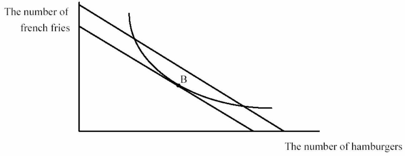
Only when Fred’s willingness to pay is just equal to what he has to pay can Fred do no better and is content staying where he is. This is a tangency between his indifference curve and his budge line:
 At point B, Fred’s best point, Fred has a tangency between his budget line and an indifference curve. Points A and C are also on his budget line, but these points make Fred less happy than does B. It is easy to see that Fred prefers B to A and C–B is on a higher indifference curve. But now you should have a better idea of WHY B is on a higher indifference curve–B is the only point on the budget line where Fred’s willingness to pay for an extra hamburger is equal to how much he has to pay. This means that at every other point on the budget line, Fred can be made better off by changing his mix of hamburgers and french fries.
So point B* is Fred’s favorite point. This looks impressive, but that’s only because if you use enough jargon and fancy graphs you might lead people to believe that you know something. Here’s another picture of Fred’s favorite point:
Look familiar? It’s the same diagram as the last one, but in this one, I’ve only drawn in what can actually be observed: Fred’s income, the price of french fries, the price of hamburgers (these three items allow me to draw the budget line), and the combination of hamburgers and french fries that Fred chooses. I can’t see Fred’s indifference curves. Evidently Fred has a tangency between an indifference curve and the budget line at B. But I can’t say anything more than that, and that is precious little. All it says is that Fred chose B because it made him happiest of all the available points. How do I know that? Because he chose it. Can I predict which point he will choose? Not unless I know where his indifference curves are. I don’t. They’re invisible until he chooses a point. I do know one thing–if he chooses his B I know the slope of his indifference curve at B. WHAT IS IT?
The picture merely says that people do what they do because it makes them happy. I have no idea in advance what makes people happy. You may have had frozen yogurt during the past week; maybe you didn’t. If you did, you had a tangency between your budget line and an indifference curve. If you, didn’t have any, evidently your highest indifference curve was where you consumed zero frozen yogurt. But I can’t tell in advance. So far, the theory of the consumer is an embarrassment. Not that embarrassing, though, given that we’ve only assumed that more is preferred to less. Knowing that more is preferred to less does tell you that Fred will consume on his budget line rather than inside it.
The Rules of the Game
The lesson so far is that people do what they do because that is what they do. This is called a tautology–something that is true by definition. In order to get some predictions about behavior we must look at how behavior changes when opportunities change. The secret is to figure out how a change in a consumer’s opportunities changes the budget line. Given the change in the budget line, can we figure out where the new tangency is? Sometimes we can say a lot about where the new tangency is, sometimes we cannot.
To be able to make predictions about behavior, you must be able to figure out the opportunities available to the individual. It will not always be obvious to you what the new opportunities are. At first you will have to guess. There is nothing wrong with guessing–the problem is knowing when you have made a good guess. Here are some rules to help you check your guesses when opportunities change:
Is there are a change in the slope of the budget line?
Remember that the slope of the budget line is the ratio of the prices of the goods. There are three ways that the slope can stay the same–prices don’t change, all prices increase in the same proportion, and all prices decrease in the same proportion. Notice in the last two cases that prices must change by the same proportion–for example, all prices going up 10%. This holds the ratio of prices unchanged, which is the slope of the budget line. All prices going up by $1.00 will not leave the ratio of prices unchanged unless all prices start out the same. SHOW THAT WHEN THE PRICE OF HAMBURGER IS NOT EQUAL TO THE PRICE OF FRENCH FRIES, A $1.00 INCREASE IN BOTH PRICES CHANGES THE RATIO OF THE PRICE OF HAMBURGER TO THE PRICE OF FRENCH FRIES, BUT A 10% CHANGE LEAVES THE RATIO UNCHANGED. Any change in price that is not in these categories must change the slope of the budget line. An increase in the price of the good on the horizontal axis must steepen the budget line. An increase in the price of the good on the vertical axis must flatten the budget line.
Is there a change in one or both of the intercepts?
Remember that the intercepts are determined by the ratio of income to the price of each good. If income changes, and the prices don’t change, the intercepts must change. There are three ways an intercept can be unchanged: income and the price of the good on that axis is unchanged, income goes up and price increases by the same percentage (why does it have to be the same percentage?), and income goes down and price falls by the same percentage. Any change in price or change in income that is not in the same percentage must change the intercept.
Is the price of the good independent of the number consumed?
In drawing the budget line so far, we have assumed that the prices the individual faces are independent of the quantity consumed. This causes the budget line to be a straight line. Later we will encounter some exceptions to this assumption.
Income Effects
Can we use the theory of the consumer to predict the effect of an increase in income on Fred’s consumption of H and F, holding the prices of the two goods constant? Let’s see. STOP RIGHT HERE. CAN YOU FIGURE OUT HOW A CHANGE IN INCOME HOLDING PRICES CONSTANT AFFECTS THE OPPORTUNITIES AVAILABLE TO FRED? USE THE THREE QUESTIONS IN BOLDFACE ABOVE. An increase in income shifts the budget line out in a parallel fashion. How do you know? The slope of the budget line is the ratio of the prices. Since these don’t change, the slope of the budget line can’t change. But the horizontal and vertical intercepts both increase. Evidently they increase just enough in both directions to result in a parallel shift:
It is important to notice that there is not a distance in the diagram that measures the change in income. The shift in the budget line represents it, but it is not a distance such as the horizontal shift in the budget line, or the vertical shift, or the shift along a diagonal line. You can read off the change in income if you know the prices by looking at the change in the horizontal or vertical intercept. The change in the horizontal intercept, for example, is the extra number of hamburgers Fred can buy, now that his income has increased. To convert that into income, you have to multiply it by the price of hamburgers. HOW WOULD YOU USE THE CHANGE IN THE VERTICAL INTERCEPT TO MEASURE THE CHANGE IN INCOME?
Where will the new tangency be?
 It is useful to divide up the new budget line as I have done in the figure. The dashed regions lie outside the indifference curve through Fred’s favorite point on his old budget line. [NOTE TO THE READER: If you are looking at the PDF version of these notes, the dashes might not show up. When referring to the “dashed region,” I’m referring to the points on the new budget line outside the arms of the indifference curve that is tangent to the original budget line at B.] A point on the dashed section of the budget line is a lower level of happiness than B–Fred prefers B on his old budget line to the dashed region. Look at the dashed region in the lower right hand corner and compare it to B. It’s true Fred gets more hamburgers in the dashed region in the lower right hand corner than he does at B, but he has so many fewer french fries that he is worse off.
Normal and Inferior Goods
With the higher level of income–the new budget line–Fred can still choose B if he wants to. He would always prefer B to the dashed region, so we know the new favorite point can’t be in the dashed region. The new favorite point must lie in between the encircling arms of the indifference curve tangent to the old budget line. Why? If Fred had a new favorite point in the dashed region, his indifference curves would have to cross. There are three possibilities in the solid region, within the arms of the old indifference curve:
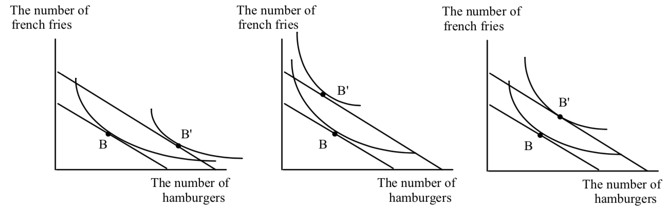 All three possibilities are consistent with the fact that indifference curves don’t cross and that they are downward sloping. In the leftmost figure, hamburgers consumption goes up and french fry consumption goes down. In the center figure, hamburger consumption goes down and french fry consumption goes up. In the rightmost figure, consumption of both goods increases.
This is not very exciting. It says that hamburger consumption goes up or down (or stays the same (this is yet another possibility I have not drawn–draw it for yourself). French fry consumption either goes up or down or stays the same. The only unambiguous prediction is that one good has to go up–they can’t both go down. This isn’t very interesting–an increase in income means that you don’t reduce your consumption on all goods. Big deal. This is not the most shining moment in the history of economic theory. (There is one other result of a change in income–an expansion of opportunities allows the consumer to get to a higher indifference curve; a reduction in opportunities forces the consumer onto a lower indifference curve. The other reason that it’s not very exciting is that because indifference curves are not observable, knowing that the new favorite point is within the arms of the indifference curves has no real observable content.)
The results shown in the figure do allow us to create some economic jargon, which turns out to be useful. If the consumption of a good moves in the same direction as the income change (income up/ consumption up, or income down/consumption down) we call the good a normal good. If consumption of the good moves in the opposite direction as the change in income we call the good an inferior good. Unfortunately, as the diagram indicates, we can’t identify a normal or inferior good until after income has changed. The terms normal and inferior are useful to describe what has already happened–they can’t be observed in advance. It is not very interesting to say that Fred’s consumption of hamburger is a normal good, unless it’s inferior. It’s like saying that the stock market is going to go up tomorrow unless it goes down. The jargon is not completely useless. The concepts of normality and inferiority will prove to be useful in helping to organize our thinking as will be seen shortly.
The Right-Angle Trick
The easiest way to observe whether a good is normal or inferior is to draw a horizontal and vertical line through the original consumption point B:
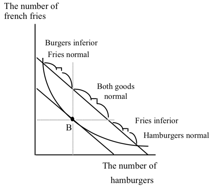
If the new tangency lies to the right of H0, hamburgers are a normal good. If the tangency lies above F0 then fries are a normal good. So if the tangency lies to within the arms of the right angle coming out of, B, both goods are normal. If the new tangency lies outside of the right-angle, one good is inferior. But as can be seen in the diagram, there is no region where the new tangency can be where both goods are inferior.
There are four common mistakes people make when dealing with income effects. The first is to misuse the right angle trick. The right angle trick identifying normality or inferiority is only for use with parallel shifts in the budget line. That is, if you want to use the right angle trick to figure out whether one or the other goods or both are normal or inferior, you can only use the right angle trick for parallel shifts.
The second mistake people make when dealing with income effects is to assume that a good is always normal or always inferior. This is not true as the figure below shows:
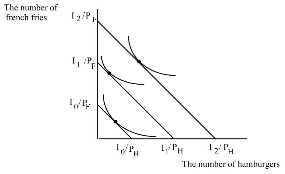
When income increases from I0 to I1, hamburger consumption goes down. When income increases from I1 to I2, hamburger consumption goes up. Hamburgers are inferior over the income range from I0 to I1 but normal over the income range from I1 to I2.
The third mistake people make when talking about income effects is to confuse the everyday meanings of normal and inferior with the economic jargon. In everyday language, normal means typical and inferior means second-rate, low-quality. But not all goods that are low-quality are inferior in the sense of economic jargon, though some may be. One of the lessons of economics is to use words carefully. Try to remember that normal and inferior have very specific meanings.
Income Effects as Expansions or Contractions in Opportunities
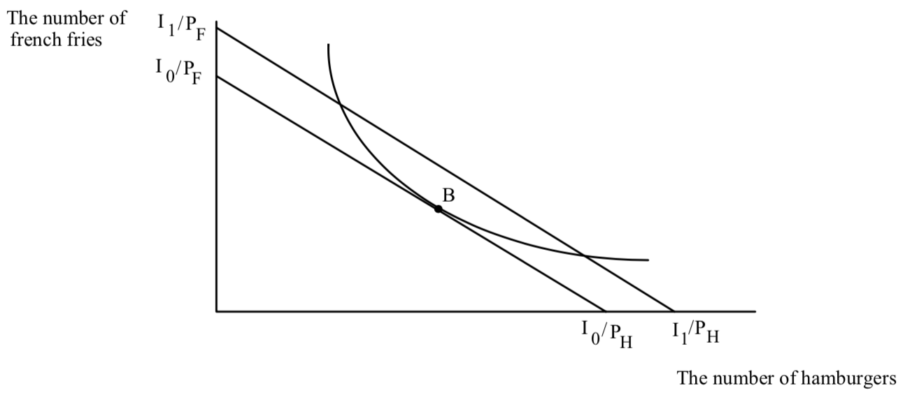
The final mistake people make when dealing with income effects is to think that they are only relevant for changes in money income. In fact, income effects are useful for describing and organizing one’s thinking about ANY change in opportunities that moves the budget line in or out and leaves the slope unchanged. What income effects are really about is how willingness to pay changes when my opportunities contract or expand. To see this, consider an increase in income from I1 to I2:
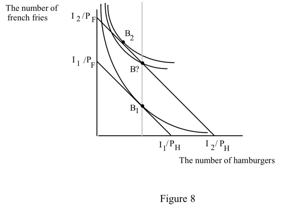 The effect of the increase in income is to move Fred’s favorite point from B1 to B2. Evidently, hamburgers are an inferior good for Fred over the range of income from I1 to I2. What does this really mean? It really tells us something about Fred’s willingness-to-pay for hamburgers when his opportunities expand. Remember that the slope of the indifference curve is Fred’s willingness-to-pay for hamburgers, measured in terms of french fries. At B1 what is Fred’s willingness to pay for an extra hamburger?
Because it is Fred’s favorite point when his income is I1, it must be the case that Fred’s willingness to pay for an extra hamburger at B1 is PH/PF.
It is possible for Fred’s favorite point when his income is I2 to be at B?. But in
fact, Fred’s indifference curve at B? is flatter than it was at B1. So the tangency in fact lies up and to the left of B?. What does this mean? What is the difference between B1 and B?? At B?, Fred has the same number of hamburgers but an increased number of french fries. Clearly, B? is on a higher indifference curve than B1. But at B?, Fred’s willingness to pay for an extra hamburger has fallen. That is why his new favorite point must lie to the left of the old one, resulting in fewer hamburgers consumed.
Saying that hamburgers are inferior for Fred over the range of income between I1 and I2 is really saying something about Fred’s preferences as his opportunities expand. It is saying that Fred’s indifference curves get flatter as you move vertically. But this is the same as saying that holding the amount of hamburgers constant while increasing the quantity of french fries, Fred’s willingness to pay for an extra hamburger FALLS. Even though Fred is getting more and more french fries as he moves in a vertical direction, he becomes increasingly unwilling to swap them for an extra hamburger. This seems a bit weird, but it is really what is going on to produce the result that hamburgers are inferior. An inferior good is a good where my willingness to pay for it falls as I get more other goods. A normal good is a good where my willingness to pay for it increases as I get more of other goods.
SHOW HOW THIS REASONING WORKS FOR THE CASE OF FRENCH FRIES BEING INFERIOR.
Even though income effects only describe what happens after the fact they are a very useful way to organize thinking about changes in a consumer’s opportunities. Suppose Fred’s income is $40, the price of hamburgers is 50¢ and the price of fries is $1. DRAW HIS BUDGET LINE BEFORE LOOKING BELOW. Suppose with these opportunities he chooses to consume 40 hamburgers and 20 fries. Now suppose his income increases to $80. The new budget line is shifted out parallel to the old one with the new horizontal intercept farther out by 80 units (WHERE DID THIS NUMBER COME FROM) and the new vertical intercept shifted out by 40. WHERE DID THIS NUMBER COME FROM?
This expansion in opportunities will result in a new favorite point for Fred which will lie along the new budget line. Suppose that hamburgers are an inferior good for Fred. The original and new situations are shown below:
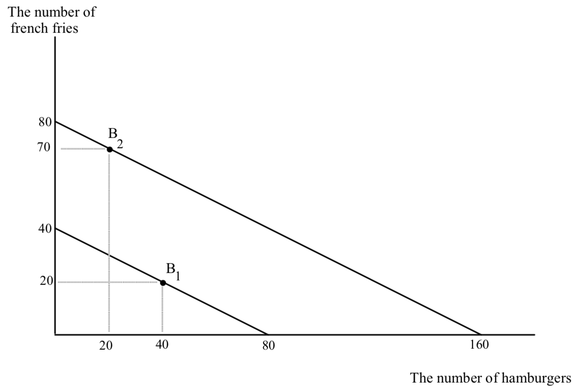 I have not drawn in the indifference curves. You can see them though can’t you, just kissing the budget lines at B1 and B2?
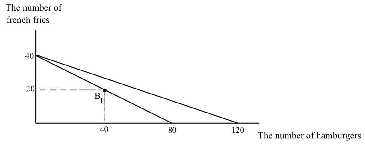
Now suppose Fred gets some bad news. His raise of $40 is canceled, so he is stuck back on his old budget line. Fred will go back to consuming 40 hamburgers and 20 french fries per week. But now Fred gets another piece of news. The price of hamburgers goes down to 25¢ and the price of fries falls to 50¢. What will happen to Fred’s consumption of hamburgers and fries? It seems like a mess. The price of hamburgers has gone down and that should increase hamburger consumption. But how will hamburger consumption be affected by the decrease in the price of fries?
But the answer is easy once you draw the budget line. The budget line when both prices are cut in half is exactly the same as when income doubled. If we already saw what Fred did when his income doubled, we can predict what he will do now when the prices (ALL of the prices) he faces are cut in half. Fred will decrease his consumption of hamburger and increase fry consumption.
A decrease in prices expands opportunities. If all prices fall or increase by the same percentage, then the slope of the budget line stays the same, and Fred’s budget line moves parallel to the old one.
Gifts as Increases in Opportunities
Here is another useful application of income effects as a way of organizing thinking. Suppose Fred is in the original situation drawn above where income equals $40, price of hamburgers is 50¢ and french fries are $1. Fred consumes 40 burgers and 20 fries. Now suppose Barney is upset that Fred is only consuming 40 burgers. He thinks that a man’s not a man unless he consumes 80 burgers a week. So every week he comes over and brings Fred enough hamburger meat to make 40 hamburgers. What does this do to Fred’s consumption of hamburgers? It seems obvious that Fred’s hamburger consumption will go from 40 to 80. But it probably won’t, and budget lines and indifference curves tell us why not.
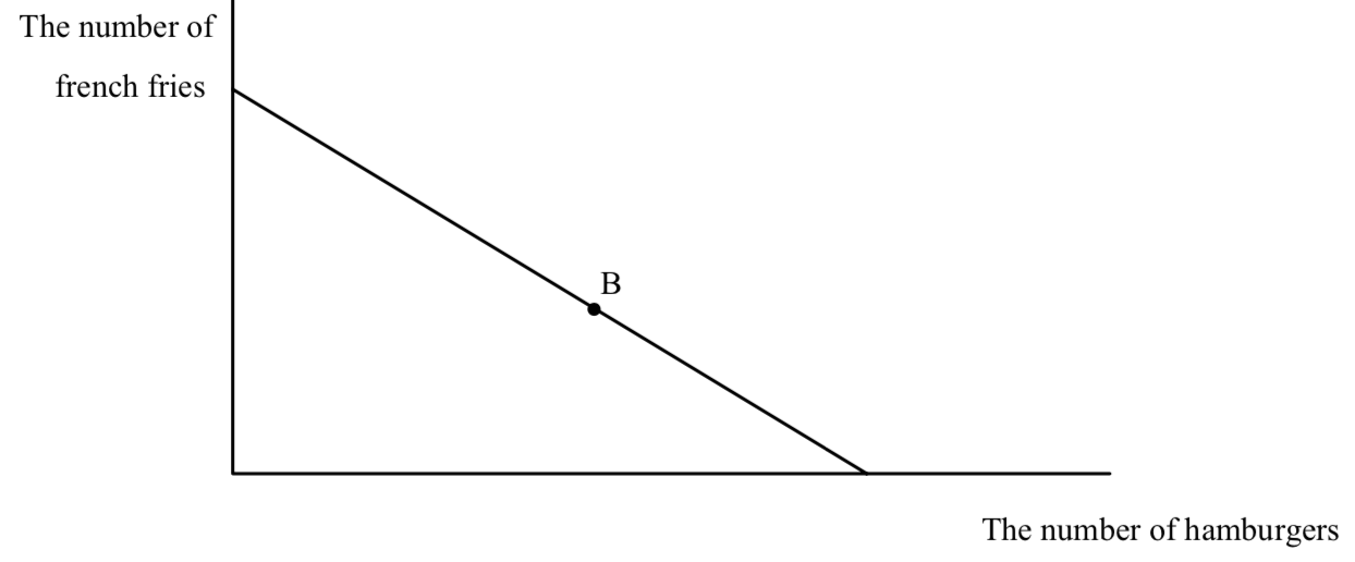
What does Fred’s new opportunities look like when he gets this gift? DON’T LOOK AT THE DIAGRAM YET! The first thing to think about is that if Fred gets the gift of 40 burgers, what happens to the maximum number of french fries and the maximum number of burgers he can consume. If Fred spends all his money on burgers he can now consume 120–the 80 he could buy with his own income and the 40 he gets from Barney. What is the maximum number of fries he can consume? If Fred spends all his money on fries he can still only consume 40. So you might think his new budget line swings out like this:
This is WRONG. Why? Don’t we have the right intercepts? We do, but it’s still wrong. To see why, look what has happened to the slope of Fred’s budget line, the way we have drawn it. The slope has decreased. Since the slope is the ratio of the price of hamburgers to the price of french fries, if figure 10 is right, either the price of hamburgers has decreased or the price of french fries has fallen. But in fact, neither has changed. You might think that hamburgers have gotten cheaper when someone gives you 40. There is a sense in which you are right, but unfortunately, it is not the way that you are thinking about it. It still remains true, even after the gift of 40 burgers, that an extra hamburger costs me 1/2 french fry. The price of hamburgers hasn’t changed.
The right picture looks like this:
The horizontal intercept is 120 and the vertical intercept is 40. The trick is being careful with how many hamburgers I can consume when I spend all my money on french fries. Before the gift, Fred had to consume zero hamburgers if he spent all his income on french fries. After the gift, if he spends all his income on french fries, Fred can consume 40 hamburgers because he will have the burgers that Barney gave him.
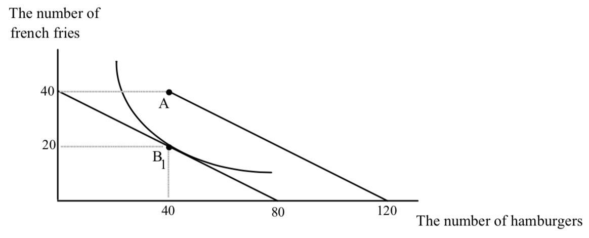
The budget line with the gift is the solid line parallel to the old budget line. Fred’s opportunities are now the point A and all the points southeast of A along the solid budget line. The parallel shift is a horizontal shift of 40 hamburgers. At any quantity of french fries consumed before, Fred can now consume an additional 40 hamburgers. What will Fred do?
The key is to notice that a gift is equivalent to an increase in opportunities. It is a parallel shift in the budget line and is almost exactly like an increase in income. (WHY DO I SAY ALMOST? WHAT IS DIFFERENT ABOUT A GIFT AND AN INCREASE IN INCOME?) A gift of 40 hamburgers when hamburgers are 50¢ is almost exactly like getting an extra $20 in income. This seems puzzling. When I get an extra $20 in income it’s clear that I can spend some of the extra $20 on french fries. How can I “spend” the extra 40 hamburgers on french fries? The answer is that the extra 40 hamburgers frees up $20 of income that I can spend on french fries. Suppose Fred is considering consuming 40 hamburgers. Before the gift this meant he could only have 20 french fries. Now, after the gift, if he wants 40 hamburgers he can now consume 40 fries. It’s like getting an extra $20 to spend on fries. The new budget line is also shifted vertically by 20 fries.
But the new budget line is not shifted vertically by 20 fries everywhere. It is only shifted vertically at quantities of hamburger of 40 and beyond. In particular, if Fred consumes zero hamburger, he can’t have 60 fries as he could if he were given a gift of $20. If Fred were given $20 instead of 40 burgers, he could also consume in a region northwest of A. We’ll return to this possibility in a minute.
There are three interesting possibilities for Fred’s favorite point in the presence of the gift:
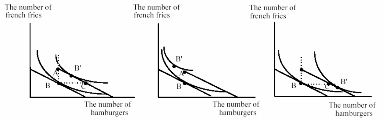 In the left-hand diagram, both hamburgers and french fries are normal goods. We know this because the new tangency after the gift, B’, is within the right angle. The result of the gift is to increase hamburger and french fry consumption, but hamburgers go up by less than 40. We know this latter fact by looking at the tangency relative to point C. At C and points southeast, hamburgers have increased by 40 or more. We know this because the horizontal distance between B and C is 40. What literally happens in the real world is as follows. Suppose the number of hamburgers at B’ in the left-hand diagram is 52. Fred takes the gift of 40, then buys 12 additional hamburgers. These 12 cost him $6. This leaves 34 dollars to spend on fries so he buys 34 fries compared to the old number of 20.
In the center diagram, hamburgers are an inferior good. If Fred had received $20, his new favorite point would be up and to the left of A. Because it’s a gift, however, he can’t get there. The highest indifference curve he will be able to get to will be the one through A which I have not drawn, but which you should be able to picture as going through A below the indifference curve through B’. What Fred would like to do is sell some of the hamburger given to him. If he can’t he will be stuck at A.
In the rightmost diagram, french fries are inferior. The new favorite point is at a lower level of fries than before. The gift induces Fred to increase his hamburger consumption by even more than the amount of the gift. At first sight this seems ridiculous–Fred is already buying 40–you give him 40 he should then consume 80. But Fred’s purchases are not fixed at 40. In this case he increases his purchases so that his total consumption exceeds 80. He could stop at 80, at point C. The fact that he doesn’t, tells us that Fred’s willingness to pay for hamburgers at point C is greater than their price, 1/2 a fry. In the same way, if Fred were given $20, he would not only spend all of it on hamburgers, he would take some of the money he used to spend on fries and use it also on hamburgers.
We can’t say what the effect of the gift will be on Fred’s consumption of hamburgers, but knowing about income effects allows to think about the gift in ways that are not obvious. An important application of the analysis is to public policy. Many government welfare programs are gifts of things rather than gifts of money. For example, the poor receive food stamps which are gifts of food. It seems obvious that giving the poor food stamps will increase their consumption of food. But it is not true, and it is unlikely that food stamps increase the food consumption of the poor by as much as the value of the food stamps. To analyze the effect of food stamps on food consumption, draw a diagram between food and all other goods. You will want to consider the effect of the following: an increase in the size of the gift, relative to the level already being consumed; whether food stamps can be sold or not; if they can be sold, whether they sell for face value or not; whether food is normal or inferior; whether all other goods are normal or inferior.
One lesson should be clear from figure 12. If the gift of food is to be different from a gift of money, the individual must be stuck at the point A, on a lower indifference curve. That is why economists tend to favor gifts of money rather than gifts of things– gifts of money maximize the happiness of the recipient while gifts of things may not. Taxpayers are not so tolerant. They prefer to see welfare recipients consume food rather than alcohol or other less desirable (in the eyes of taxpayers) items. What do you think?
Try to keep separate the rights of taxpayers, what they ought to do, and what they actually do. These three ideas are not always the same.
Changing the Price of Hamburger, Holding Income and the Price of Fries Constant
Changes in income have ambiguous effects on changes in consumption. This is disappointing, but at least income effects are useful ways to organize thinking. Now let’s look at a change in the price of hamburger. Surely a decrease in the price of hamburger holding income and the price of fries constant will unambiguously lead to an increase in hamburger consumption. Unfortunately, it does not. STOP. HOW DOES A CHANGE IN THE PRICE OF HAMBURGER, EVERYTHING ELSE HELD CONSTANT, CHANGE OPPORTUNITIES? A decrease in the price of hamburgers holding income and the price of fries constant pivots the budget line, where the pivot point is the vertical intercept. We know the vertical intercept doesn’t change–the vertical intercept is determined by income divided by the price of fries–we are holding these constant so the intercept doesn’t change. The horizontal intercept does change–it increases because the price of hamburgers has fallen. THERE IS A TENDENCY TO GET CONFUSED HERE–A DECREASE IN THE PRICE OF HAMBURGERS INCREASES THE HORIZONTAL INTERCEPT. The slope of the budget line decreases–the price of hamburgers has fallen so the slope which is the ratio of the price of hamburgers to the price of fries, is lower. The effect on opportunities is shown below:
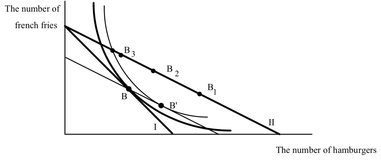
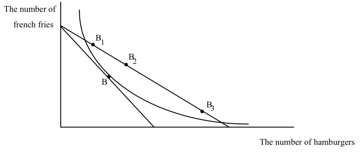 The favorite point on the original budget line is point B. The new budget line is flatter. I have shown three possible new favorite points, B1, B2, and B3. All three are possible, since it is possible to draw in tangencies at any of the points where indifference curves will not cross the original one through B. Horrifying though it may seem, the effect of a decrease in the price of hamburger can lead to a decrease or an increase in hamburger consumption. We will return to the effect of a change in the price of hamburger in a bit. Before we do it is useful to find the only unambiguous prediction of the theory of the consumer.
Twists in the Budget Line–The Only Unambiguous Result of Consumer Theory
Fortunately for mankind and economists, there is an unambiguous result from the theory of the consumer. So far we have looked at parallel shifts and pivots in the budget line. Now consider a twist in the budget line where the twist is through the original favorite point.
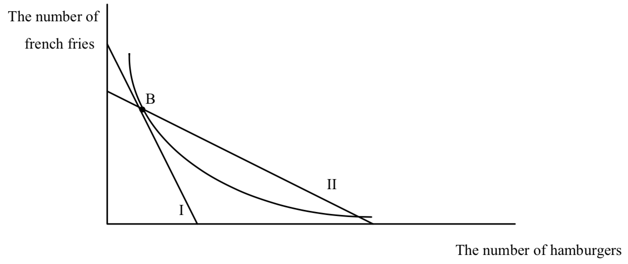 The original budget line is budget line I. The new budget line goes through the old favorite point, B, but is flatter. Where is the new favorite point? The new favorite point is again found somewhere on the new budget line somewhere inside the arms of the old indifference curve through B. But this region is always down and to the right of B– an increase in hamburgers and a decrease in fries relative to B. An unambiguous prediction! Any point on budget line II where hamburger consumption decreases, can’t be a tangency because indifference curves would have to cross.
Now consider a twist through B where the budget line gets steeper:
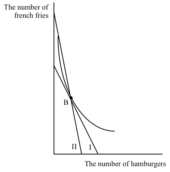
The new budget line, II goes through B and is steeper. The new favorite point is again in an unambiguous region–up and to the left of B where hamburgers must decrease and french fries must increase.
What Twists the Budget Line?
Let’s start with twists that are flatter, figure 14. What will twist the budget line through the old favorite point but with a flatter slope? One answer is any change in opportunities that lowers the price of hamburger but that still allows Fred to buy the old combination of hamburgers and french fries at B. A numerical example will help. Suppose the price of hamburgers is $1, the price of french fries is $2, and Fred’s income is $40. Let’s assume that Fred chooses to consume 12 hamburgers and 14 french fries when he faces these prices with his income. Now let’s find a change in opportunities such that his new budget line is flatter but passes through B. Here’s one: a change in the price of hamburger to 50¢ with a simultaneous reduction in income of $6.
First, let’s see that the new budget line is flatter. The price ratio has fallen from 1/2 to 1/4, so the budget line is indeed flatter. Now let’s see whether Fred can still consume his old combination of 12 hamburgers and 14 french fries given that hamburgers are cheaper but at the same time his income is only $34. The 14 french fries still cost him $28. The 12 hamburgers cost him $6 at their new price of 50¢, so he can buy the old combination. In fact he can just buy it, with no money left over, so his new budget line must pass through B with a flatter slope. Another way to see this is that with the new price of hamburgers, the old combination is now $6 cheaper. Taking away the savings of $6 just allows Fred to consume the old combination:
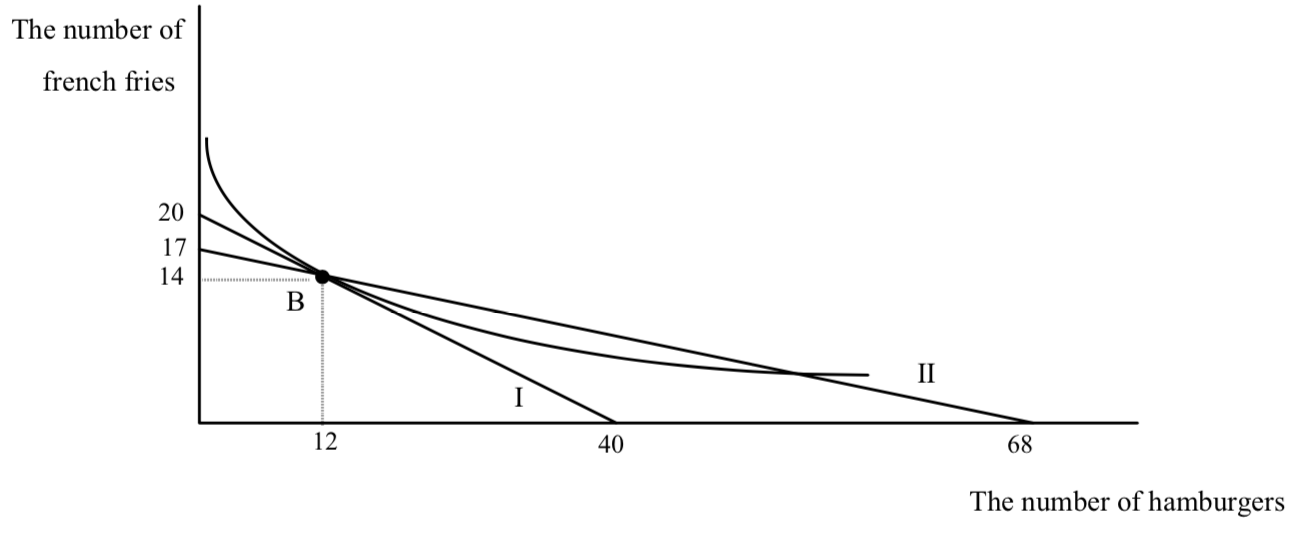 (You should verify that the new horizontal intercept is indeed 68 and the new vertical intercept is indeed 17.) Fred’s new favorite point must be southeast of B. The effect of a twist is to increase his consumption of hamburgers and decrease his consumption of fries.
We call the effect of a twist the substitution effect. The substitution effect is a change in the slope of the budget line that still allows the consumer to consume the original consumption point. Rather than continuing to write the phrase “that still allows the consumer to consume the original consumption point”, we say that “holds purchasing power constant.” Fred’s purchasing power is maintained in figure 16 because he can still purchase his old bundle if he wants to.
One way for a twist to occur is for a price to change, and for income to change in the same direction by enough to hold purchasing power constant. What is the amount of income that holds purchasing power constant? In the case of a decrease in the price of hamburgers, it is the amount of income you can take away and still enable me to buy the old combination of hamburgers and french fries. Let’s see what that amount is. Remember the equation of the budget line:
I = pHH + pFF
This equation must hold at H0 and F0, the original quantities of H and F before the price of hamburger decreases. Let pH0 be the original price of hamburger, and let pH1 be the new price. Since the price of hamburger has decreased, if I buy the old amount of hamburgers, H0, expenditure on hamburger will decrease. What is the change in expenditure:
pH1H0 – pH0H0 = (pH1 – pH0)H0
The income change necessary to hold purchasing power constant when the price of a good changes is just the change in the price of the good multiplied by the amount of the good originally consumed. When the price of hamburger falls, pH1 is less than pH0. So the change in income is negative–you must take away income from Fred when the price of hamburger falls in order to holds purchasing power constant. When the price of hamburger increases, pH1 is greater than pH0. So the change in income is positive–you must give Fred income when the price of hamburger increases in order to holds purchasing power constant.
The substitution effect is the only change in the consumer’s opportunities that has an unambiguous effect. THE SUBSTITUTION EFFECT ON QUANTITY IS ALWAYS IN THE OPPOSITE DIRECTION FROM THE CHANGE IN PRICE. Here, the price of hamburgers has fallen and the quantity of hamburgers consumed increases.
Strangely enough, a change in the price of FRENCH FRIES can also create the same opportunities as a change in the price of hamburger. Suppose the price of french fries goes from $2 to $4 with the price of hamburger at its old level of $1. Let’s hold purchasing power constant again–let’s find the change in income that will allow Fred to buy the old bundle of 14 fries and 12 burgers now that fries have gotten more expensive. Because the price of one of the goods has increased, Fred will require an increase in income to allow him to buy the old bundle. How much extra income? The new bundle is going to cost an extra $28. So if Fred has $68 ($40 + $28) he should be able to buy the old bundle at the new prices.
But look at the new budget line when Fred has income of $68, and faces a price of hamburgers of $1 and a price of french fries of $4. The horizontal intercept is 68 hamburgers and the vertical intercept is 17. The slope is 1/4. This is the same twist as in figure 16.
An increase in the price of french fries that holds purchasing power constant has the exact same effect on opportunities as a decrease in the price of hamburgers holding purchasing power constant. As a result, Fred’s new favorite point, B’, in the region southeast of B within the arms of the indifference curve, is the same in both cases. This may seem incredible, but the intuition is as follows: in both cases, whether the money price of french fries goes up or the money price of hamburger goes down, Fred can stay at B if he wants to. But he won’t want to. The value to Fred of an extra hamburger at B hasn’t changed. But the price has fallen. It used to be that Fred had to give up 1/2 a french fry to get an extra hamburger. Now he has to only give up 1/4. So he will substitute towards the good that has gotten cheaper and away from the good that has gotten more expensive. (Notice that this is the same intuition we used to show that A couldn’t be Fred’s favorite point back a few diagrams ago.)
When the money price of hamburgers decreases or the money price of french fries goes up, in both cases hamburgers are cheaper in the essential meaning of cost: how many fries do I have to give up to get another hamburger. The substitution effect highlights the importance of relative prices not absolute prices as the determinant of behavior.
Isn’t the Substitution Effect Kind of Hokey?
The substitution effect sure looks hokey. I’ve told you that there is one unambiguous result in the theory of the consumer and it turns out to be this weird combination of a change in price and a change in income at the same time. Why should these things happen together? What if they don’t? Are we left stranded?
Despite the weird and arbitrary appearance of the substitution effect it is extremely useful in thinking about all kinds of situations. Remember, anything that twists the budget line holding purchasing power constant causes the substitution effect to occur. Here are some applications, from the ridiculous to the sublime, that will show you the usefulness of the substitution effect and help you understand how it works.
Discount Beer and the Cover Charge
Joe College’s favorite bar is called Brewski’s. At Brewski’s, beers are $2.50 and bags of pretzels are $1. Joe goes to Brewski’s every Saturday night with $10 and has to decide how many beers to drink and how many bags of pretzels to eat. Suppose he drinks 2 beers and eats 5 bags of pretzels. Illustrate Joe’s decision. Draw his budget line, and draw in an indifference curve tangent to the budget line at 2 beers and 5 bags of pretzels. One Saturday night, Joe arrives at Jimmy’s and finds out that there is a special deal for economists. Joe, being an economist, is thrilled. On Economist Night, beers are only 50¢. Unfortunately, there is a cover-charge of $4 to get in.
Should Joe admit that he is an economist? If he does, will he consume, more, less, or the same amount of beer on Economist Night compared to a regular Saturday night? What will happen to pretzel consumption? Isn’t it horrifying to think that the substitution effect, the only unambiguous result from the theory of the consumer is best applied to drinking in a bar? Well, no–it turns out that Economist Night will give us a lot of insight into subsidies.
What will happen to Joe on Economist Night? He has a different set of opportunities. The price of beer has fallen, but so has the money available to spend on beer and pretzels because of the cover charge. Think. Does this story sound familiar? A decrease in price and a decrease in income. Could be the substitution effect. Let’s see. For this to be the substitution effect purchasing power must be held constant. Remember that for purchasing power to be held constant, income must change in the same direction as price and be equal to the change in price multiplied by the original amount of consumption of the good whose price changed. In this case, the price of beer fell by $2 and the original number of beers consumed was 2. Voila! The cover charge, the reduction in Joe’s income, $4, is exactly equal to the right amount to hold purchasing power constant.
Given that Joe’s originally consumes 2 beers, a $2 reduction in the price of beer accompanied by a $4 reduction in Joe’s income, will flatten Joe’s budget line (assuming we put beer on the horizontal axis) and hold purchasing power constant. Joe will consume more beers, fewer pretzels, and be on a higher indifference curve than he was before. So it will be in Joe’s interest to declare himself an economist–by qualifying for economist night, he is better off. If you are catching on, you can see the graph behind the preceding sentences without drawing it. If you’re not catching on, you should be able to figure it out by drawing the graph. If you can’t draw the graph, re-read the previous stuff and try again. We’ll draw the graph now without you and you can come back later when you’re ready to draw it for yourself. We’re drawing the graph because it will come in handy to understand why this problem has a wider application.
Joe’s original situation is shown in bold. His situation on economist night is shown in the lighter line with outlined numbers (12):
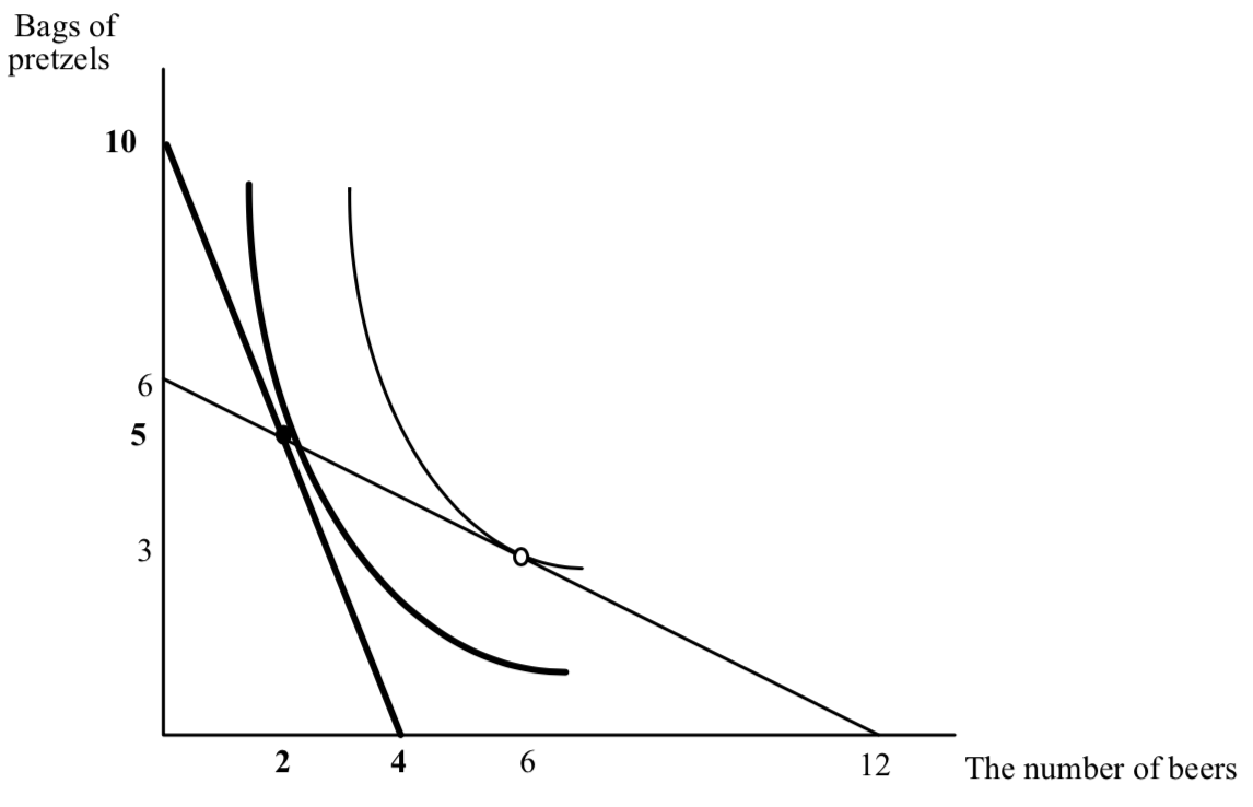 First check the vertical intercepts in the original situation–price of beer $2.50, price of pretzels, $1, income $10. The horizontal intercept is 4 and the vertical intercept is 10. On Economist Night, price of beer is 50¢, price of pretzels is still $1, income, after cover charge, is $6. Horizontal intercept is
 , vertical intercept is . The budget line on economist night is flatter because the ratio of the price of beer to the price of pretzels has fallen from 21/2 to 1/2. Given his opportunities on Economist Night, Joe substitutes towards beer and away from pretzels–beer consumption increases to 6 and pretzel consumption falls to 3. So even though Joe can stay with the same consumption that he had on non-Economist Night, he won’t–he can do better by substituting towards beer and away from pretzels.
(You might also think about Economist Night from the perspective of the bar. Here is a bad mistake in reasoning: “Economist night is a great idea–Joe is better off, and the bar owner breaks even. The bar owner used to collect $10 dollars from Joe, and on economist night he still does. So Joe is better off, and the bar owner is indifferent.” This is WRONG. What does it ignore? It ignores the fact that while the bar owner does collect $10 from Joe, he has to sell him 6 beers and 3 bags of pretzels to do so. Remember that in competition, the price of an item is equal to marginal cost. If the bar is competitive, the owner will lose $2 on every beer he sells to Joe. (In fact he will probably lose more than two dollars on each beer. Do you know why?) So it costs the bar owner an additional $12 to increase Joe’s happiness.
This leads to two interesting questions. Is Joe made happy enough to bribe the owner to lower the price of beer? (Is there a cover charge that will induce the owner to lower the price of beer?) If cover charges lower the profits of bars, why do so many bars have cover charges? We will return to answer these questions later on.)
The Story of the Farmer
Consider a farmer, who each week grows 20 potatoes and five pounds of hamburger meat, enough to make 10 half pound hamburgers. We will assume that he is stuck growing these amounts, and that he is able to grow them at zero cost. After finishing the discussion of the farmer, you might wonder why I assumed that the farmer’s output is not under his control. The farmer only likes meat and potatoes. He can eat what he grows, or he can sell it in the market. Suppose the market price of beef is $2 per pound, or $1 per hamburger, and the market price for potatoes is $1 per potato. Will the farmer sell some of his meat to get more potatoes? Will he sell some of his potatoes to get more meat? Or will he do neither and eat exactly what he grows?
All three situations are possible. To see this, think about the farmer’s opportunities for consumption. One point is certainly on his budget line–the point 20 potatoes and 10 hamburgers. In addition he can sell all of his hamburgers, get $10 and use the money to buy 10 potatoes. So his maximum number of potatoes is 30. Alternatively, he can sell all of his potatoes, get $20 and buy hamburger meat, enough for 20 more hamburgers. His budget line is shown below:
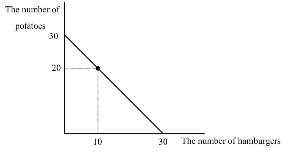 Where he consumes, depends, as always, on where his indifference curves are tangent to the budget line. If they are tangent to the budget line to the northwest of the 10, 20 point, the farmer will sell beef and buy potatoes. If the tangency is to the southeast of the 10, 20 point, the farmer will sell potatoes to get more beef. Let’s assume that the farmer arrives at the market, observes the prices of beef and potatoes, considers his preferences for eating them and decides to make no transactions in the market–he eats exactly what he is able to produce. This means his tangency is right at the combination 10, 20.
The farmer returns to the market a week later. Before looking at the diagram below, think about which situation the farmer would prefer, an increase in the price of potatoes or a decrease in their price. Incredibly, either case makes him better off. Why? Both changes cause a substitution effect. Purchasing power will be held constant because whether the price of potatoes goes up or down, the farmer will be able to still consume his old combination of 10, 20. The key insight is given that purchasing power is held constant, either an increase in the price of potatoes or a decrease in the price of potatoes makes one of the goods cheaper to consume and allows the farmer to increase his happiness by shifting his consumption towards the good which has gotten cheaper.
It’s clear that when the price of potatoes falls, potatoes have gotten cheaper. But when the price of potatoes increases, hamburgers have gotten cheaper, just as in the case discussed above:
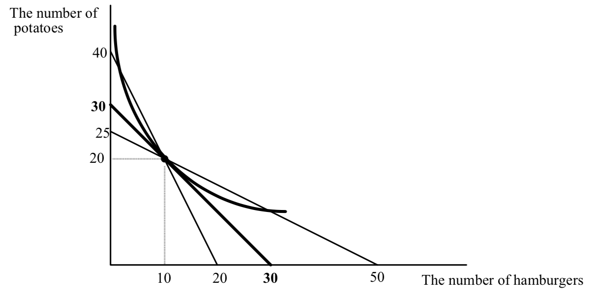
The original situation is shown in bold. The new situations, where the price of potatoes has fallen to 50¢, or increased to $2 are shown in lighter print. When the price of potatoes decreases, the budget line goes through B and becomes steeper. It is the line with horizontal intercept 20, and vertical intercept 40. You can think of either potatoes getting cheaper or hamburgers getting more expensive. Hamburgers are more expensive when the price of potatoes falls to 50¢ because now every hamburger eaten costs 2 potatoes when they used to only cost 1. The farmer will substitute away from the good that has gotten more expensive (hamburgers) and towards the good that has gotten cheaper (potatoes).
When potatoes get more expensive, the budget line twists through B and gets flatter, just as if the price of hamburgers had fallen. Hamburgers have gotten cheaper, in the real sense that consuming an additional hamburger only costs 1/2 a potato when the money price of potatoes goes to $2. You probably find this intuitive. What is unintuitive is that this increase in the price of potatoes actually makes the farmer happy. The intuition is that an increase in the price of potatoes not only makes consuming a hamburger less expensive, it expands the farmer’s ability to eat hamburgers as well–his horizontal intercept increases. And that is because the farmer comes to the market with 20 potatoes. When potatoes are $2, the potato eater is sad. But the potato seller is glad– the income potential of the potatoes has increased. The increase in the price of potatoes induces the farmer to sell some of the potatoes he used to eat, and convert them into hamburgers.
You might think that the farmer doesn’t care what the prices of potatoes and beef are since he grows them without cost. But they each have an opportunity cost. Eating a potato has a cost even when growing it does not–the cost is the hamburgers that could be purchased with the money from selling the potato.
To see if you understand the story of the farmer, ask yourself which he prefers, an increase in the price of beef or an increase in the price of potatoes. The answer is that it doesn’t matter–either change will make him better off as long as he is originally at B. You might think that because at B he is consuming 20 potatoes and “only” 10 hamburgers, he likes potatoes more than hamburgers, but this is false. Do you know why? ANOTHER WAY TO SEE WHAT IS GOING ON WITH THE FARMER IS TO TURN THE FARMER INTO A TYPICAL CONSUMER WITH A FIXED INCOME AND FACING PRICES OF BOTH GOODS. WHEN THE FARMER COMES TO THE MARKET, HE SELLS ALL OF HIS PRODUCE, THEN TAKES THE MONEY AND ALLOCATES IT BETWEEN HAMBURGERS AND POTATOES. SHOW THAT YOU GET THE SAME EFFECTS ON THE BUDGET LINE AND THE CONSUMPTION CHOICES OF THE FARMER.
The farmer story should help you understand the cover charge story, and the general effect of price changes in the presence of taxes. You might think that when Joe goes to the bar and sees the cover charge he says to himself–“Every Saturday night I come to the bar and I spend $10. Now with this cover charge and price reduction on beer, I can still consume the same quantities of beer and pretzels that I did before.
Great!” Joe might say that, but if he did, he’s not very smart. It’s true he can still consume the same quantity he did before, but why should he? He can be even happier by increasing his beer consumption. Think about the farmer. He can go through life consuming 10 hamburgers and twenty potatoes. But suppose somebody discovers that if you live in a city, potatoes help reduce your risk of cancer. The demand for potatoes will increase and the price of potatoes will increase. Is it smart for the farmer to keep eating the same mix when potatoes are $4, say, instead of $1? (WHY DID I ASSUME THAT POTATOES ONLY REDUCE THE RISK OF CANCER FOR PEOPLE IN THE CITY?)
A similar related mistake is to assume that Joe always spends $10 on beer. Life doesn’t work that way. Joe may show up at the bar every Saturday night with $10 in his right pocket to spend on beer, the rest of his money in his left pocket to spend on all other goods. He shows up at the bar and finds he has to pay a $5 cover charge. He could say, “I’ll use the money in my right pocket to pay for the cover charge and I’ll spend the remaining $5 on beer regardless of the price of beer. Won’t his consumption of beer depend on the price?
The Effect of a Price Change Holding Money Income and Other Prices Constant
Earlier we looked at the case where the price of hamburger decreased, while money income and the price of fries stayed the same. Let’s return to that case, and see how the substitution effect can be used to help understand it:
The original budget line, budget line I, is shown in bold. The new budget line is the flatter bold line, II, pivoting out of the french fry intercept. The french fry intercept doesn’t change. WHY? The original best point is B. Budget line II is a lot like the substitution effect–hamburgers have gotten cheaper. The budget line is flatter. The difference is that a change in the price of hamburger holding other prices and income constant does not hold purchasing power constant. Purchasing power has increased. Before the price change I could just afford B. Now if I buy the bundle B I have money left over.
How can I have money left over if my income hasn’t changed? If I consume the old bundle, the decrease in the price of hamburger frees up income I used to spend on hamburger. It’s a lot like getting more income. But it’s not just like it. With an income change my budget line shifts out parallel. The move from budget line I to budget line II is not a parallel shift. It is not a parallel shift because the expansion of opportunities caused by the price change depends on how many hamburgers I consume. If I consume a lot of hamburgers, a decrease in price expands my opportunities a lot. If I consume a few, the expansion in opportunities is small. That is why the vertical distance between the two budget lines grows as I increase the number of hamburgers.
So a decrease in the price of hamburger holding income and the price of fries constant expands my opportunities. It also changes the price at which I can exchange hamburgers for french fries. Sounds like a combination of a substitution effect and an income effect. It is. The light budget line shows the substitution effect if the decrease in the price of hamburger fell but without holding income constant. If we let income change just the right amount to hold purchasing power constant, we get the substitution effect. We know how much income that is–the old quantity of hamburgers multiplied times the change in the price of hamburgers. That amount of income is a measure of the increase in purchasing power from the decrease in the price of hamburger. (WHICH WOULD THE CONSUMER RATHER HAVE–A DECREASE IN THE PRICE OF HAMBURGER, OR THE INCREASE IN INCOME EQUAL TO THE PRICE DECREASE TIMES THE OLD QUANTITY OF HAMBURGERS.)
To understand the effect of the change in the price of hamburgers holding the price of fries and income constant, think of it as a two-step move–a twist (the substitution effect) and a parallel shift. The twist moves the consumer to B’–hamburgers increase and fries decrease. The effect of the parallel shift, the expansion in opportunities is, like the effect of any change in income, uncertain. If hamburgers are a normal good, the income effect of the price change reinforces the substitution effect and moves us to a point like B1. If hamburgers are inferior, there are two possibilities. At B2, hamburgers are inferior, but not so inferior that the income effect outweighs the substitution effect. At B3, hamburgers are inferior, and so inferior that the income effect outweighs the substitution effect.
Let’s look at this last possibility a little more closely. How can a decrease in the price of hamburger cause a person to consume less hamburger? This means that Fred has an upward sloping demand curve for hamburger. The intuition is that yes, the decrease in the price of hamburger by itself tends to increase hamburger consumption. But the decrease in the price expands opportunities. Fred may choose to use his expanded opportunities to buy a lot more fries and less hamburger so that the net effect is a decrease in hamburger consumption.
When the price of a good changes holding income and the price of other goods constant and the consumption of hamburger moves in the same direction as the change in the price (price falls, hamburger consumption falls, price increases, hamburger consumption increases) we call the good a Giffen good. Giffen goods must be inferior, but not all inferior goods are Giffen goods. Giffen goods are possible but none has ever been measured statistically for an entire market. There are two reasons for this. First, the typical good consumed by the consumer is normal. HOW DO I KNOW THIS? Second, and most importantly, Giffen goods require radical changes in willingness to pay for small changes in consumption. To see what I mean by this, look at the figure and look at two points–B3 and the point just to the northwest of B3 where the new budget line crosses the substitution effect indifference curve. Draw the indifference curve that is tangent to budget line II at B3. It’s hard to draw without having it cross that other budget line. It has to curve away very steeply. Now compare the slope of that indifference curve at B3, with the slope of the indifference curve at the unlabeled dot right next to it.
The slope are very different. But that means that at the unlabeled dot, Fred is willing to pay a lot more to get one more hamburger, than he is at B3. (If you’ve forgotten how to interpret slopes of indifference curves, go back to the opening section.) But B3 and the unlabeled dot are almost right next to each other. Why would somebody’s value of an extra hamburger change so radically when he had a slightly different mix of hamburgers and french fries.
If you choose Fred’s original point B at different parts of the original budget line, I, you will find that as Fred’s original point is farther to the northwest (which means that as he consumes less and less hamburger in the original situation, it gets harder and harder to squeeze in a Giffen good tangency without having the indifference curves cross. It can always be done, but you will find that the change in slopes of indifference curves at nearly adjacent points become more and more divergent. Try it. This is why Giffen goods become increasingly unlikely as the proportion of income devoted to a good falls.
A Closer Look at Subsidies
Suppose the government wants to increase the consumption of bread. Bread is currently $1. The price of AOG is also $1. The government offers a 50¢ rebate to consumers for every loaf purchased. Assume that the supply curve of bread is horizontal so that the price suppliers receive stays at $1. The price demanders pay will fall to 50¢. For those consumers of bread who pay no taxes, the effect of the subsidy is to decrease the slope of the budget line, as shown in the last figure, increasing bread consumption as long as bread is not a Giffen good.
Government must raise taxes to pay for the rebate. The rebate causes a deficit equal to .5 ∑ Bi, where Bi is the amount of bread purchased by consumer i, and the summation is over all consumers of bread. There are lots of ways to allocate the taxes necessary to pay for this plan. Consider two extreme plans.
Plan I:
Under Plan I, the government sends you a rebate check at the end of the year. The size of the check is the number of loaves of bread you have consumed during the year multiplied by 50¢. At the same time the government sends you a tax bill. The tax bill is equal to the size of your rebate check. For someone who consumes 50 loaves a year, the rebate check is $25 and the tax bill is also $25. This insures the government collects enough money to pay for the subsidy rebate.
Plan II:
Under Plan II, the check you receive from the government is determined in the same way as in Plan I–you get 50¢ for every loaf consumed. Your tax burden is determined differently. To balance the budget, the government takes the deficit of .5 ∑Bi, and divides it equally among all consumers of bread. Suppose there are n consumers.
Then each taxpayer receives a tax bill of (.5∑Bi)/n. Since there are n consumers, total taxes collected just equal .5∑Bi, so again, the government has just enough money to pay for the budgetary cost of the subsidy.
We would like to know how these two plans affect the opportunities of consumers and if they make consumers better off or worse off. Let’s start with Plan I first. Plan I has no effect on the consumers budget line. His original opportunities are given by his budget line:
I = pBB + pAA
where pB is the price of bread, pA is the price of all other goods, B is bread consumption,
and A is consumption of all other goods. Because the initial price of both goods are 1, the budget line can be written as:
I = B+ A
Under Plan I, income is augmented by .5 for every loaf of bread consumed, but decreased
by .5 to pay for the tax bill:
I-.5B + .5B = B + A
or
I = B+A
the same budget line as before. This is not surprising, since bread has not gotten any
cheaper in any real sense. Now consider plan II.
Under plan II, income is increased by .5 for every loaf of bread consumed, and decreased by .5Ba, where Ba is equal to (∑Bi)/n, the average number of loaves
consumed. So the budget line can be rewritten as:
I + .5B – .5Ba = B + A
or
I – .5Ba = .5B + A
or
I’ = .5B + A
where I’ is equal to the original income minus .5Ba. The new budget line under plan II, is twice as flat as the old one, but has less income. So the budget line pivots then shifts in parallel. It sounds a lot like a twist in the budget line, the Slutsky substitution effect. Let’s see if it is.
In order to see the effect on consumption and happiness, we have to specify whether the person we are looking at consumes more than, less than, or exactly the same amount as the average. One way to think of Plans I and II is to think of them as the government sending you two letters at the end of the year. In the first letter is a check for an amount equal to 50¢ times the number of loaves you consumed during the year. In the other is your tax bill–your share of the money necessary to finance the payments in the other letter. Or you can think of the combination subsidy/tax program as a single program. At the end of the year, the government sends you a single letter–either a bill, a check, or a note that says you neither owe nor will be subsidized. Under Plan I, everyone gets the latter note because everyone’s tax bill is set equal to their subsidy check. Again, it would then be kind of obvious that there was no real subsidy.
The weird thing is that under plan II, the following holds:
- Everyone faces a lower price of bread, even people whose letter at the end of the year contains a bill.
- If there is a person who happens to consume the average amount of bread, and who at the end of the year receives a note that says he neither owes nor receives money, this person also faces a lower price of bread and is worse off after the subsidy/tax program.
- Even some people who receive positive checks at the end of the year are worse off.
To see the effect of the subsidy, consider a person who receives only the subsidy of 50¢ per loaf and bears none of the tax. This person is represented in the figure below. The effect of the subsidy alone is to flatten the budget line–it pivots out from the AOG axis:
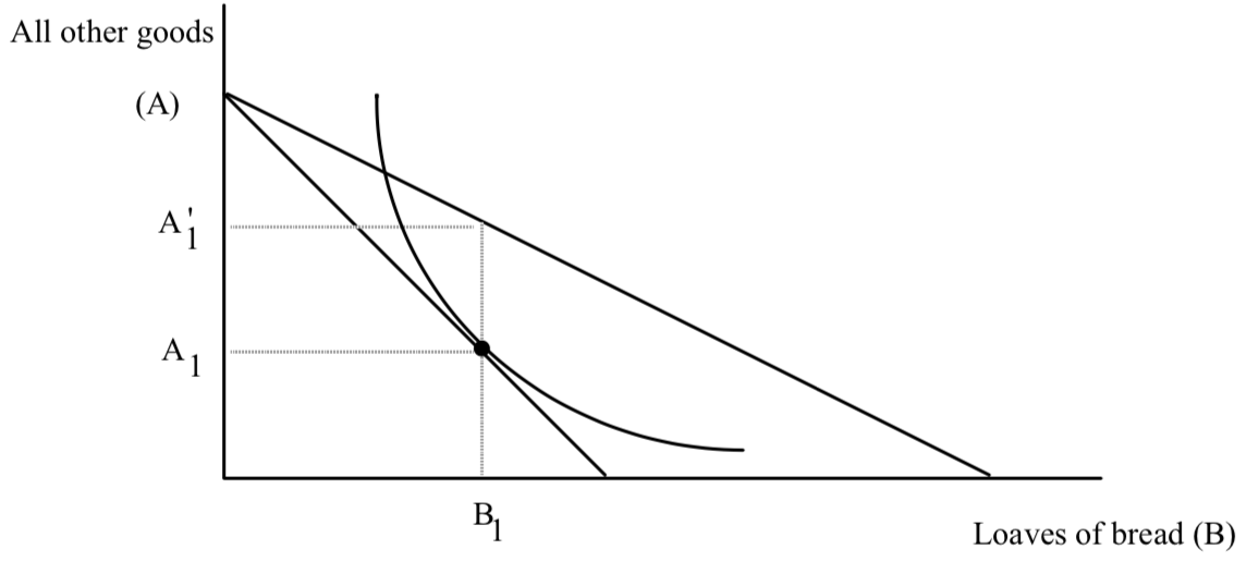
Before the subsidy, the consumer shown chose to consume B1 loaves of bread and A1 units of all other goods. Now with the subsidy, if he continues to consume B1 loaves of bread, he can now have more of all other goods–A1′ units. This is true at every quantity of bread except zero. The vertical distance between the two budget lines represents the extra amount of all other goods the consumer can have by virtue of the subsidy plan. But since the price of all other good is $1, the vertical distance between the two budget lines represents the check the government sends the consumer at the end of the year. Notice that the vertical distance between the two lines grows as the number of loaves consumed increases, which makes sense–as the number of loaves consumed increases, the size of the check increases. You can also show that for every quantity of bread, the vertical distance is .5 times the quantity of bread.
The fact that the check is tied to one’s own bread consumption in a positive way– the more bread consumed, the bigger the check–is what makes bread cheaper. This is reflected in the budget line as a flattening.
Now consider the effect of the tax. The government is going to tax all individuals the same amount–an amount equal to the 50¢ times the average amount of bread consumed. The government can measure the average amount of bread consumed before the program exists. But the government will not know in advance what the average amount consumed will be when people face the combination subsidy/tax scheme. They make an estimate. If the estimate is too low, the program will run a deficit. If the estimate is too high, the program runs a surplus. And remember–the size of the tax affects the average. Suppose the government finds out that when it sets a tax of $20, the average number of loaves consumed is 40. Then the program is in balance.
Let’s see how the subsidy combined with the tax affects behavior and happiness. Consider Jean, a consumer who consumed 40 loaves of bread BEFORE the program. What will be the effect of the program on his behavior? In Jean’s case, we know exactly what happens to his budget line–it has a slope of 1/2 and it goes through his original consumption point of 40 loaves of bread and whatever is the old level of AOG.
The combination of the tax and subsidy holds Jean’s purchasing power constant. He can stay at 40 loaves and the old amount of AOG, but he won’t because of the intuition of the substitution effect. A twist in the budget line that flattens it induces Jean to buy more bread and less AOG as shown below:
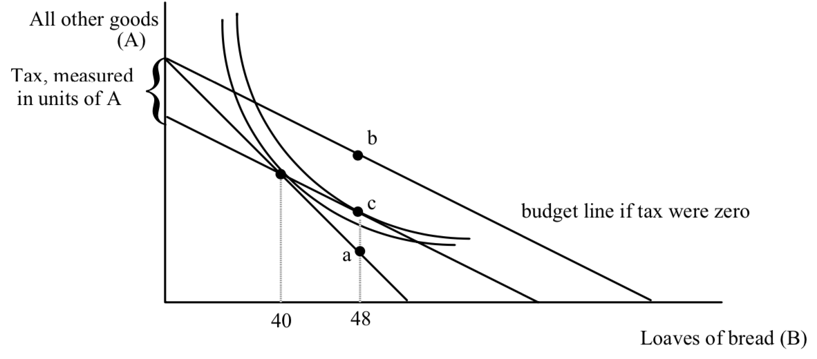
Jean substitutes toward bread and ends up at c. We know that c is to the southeast of the original point. As a result, we know that Jean’s net result from the government must be a check rather than a bill or a note saying he neither owes nor receives. We know this because Jean would get the neutral note if he ended up consuming the average, 40. But Jean consumed 40 loaves BEFORE the program existed. He consumes more now because the combination of tax and subsidy is a twist increasing bread consumption. His subsidy check must exceed $20. So the net impact of the subsidy and the tax is a check at the end of the year. As I have drawn Jean’s indifference curves, he gets a check of $4 at the end of the year.
If we think of Jean receiving a subsidy check and a tax bill rather than a single consolidated statement, his subsidy check is the vertical distance between points a and b, his tax bill is the vertical distance between points b and c, and $4 is the vertical distance between a and c–the increase in purchasing power net of both parts of the government program. The vertical distance between a and c is the vertical distance between his original budget line and his new net budget line when he faces the tax and receives the subsidy, given that he consumes 48 loaves of bread–it is the extra AOG he can consume at 48 loaves of bread, above and beyond what he could have consumed before the program existed.
Jean is better off from the program. But if there is someone who ends up consuming an amount of bread exactly equal to the average, 40 loaves, he will not look like Jean. He will look like Javert, as shown below:
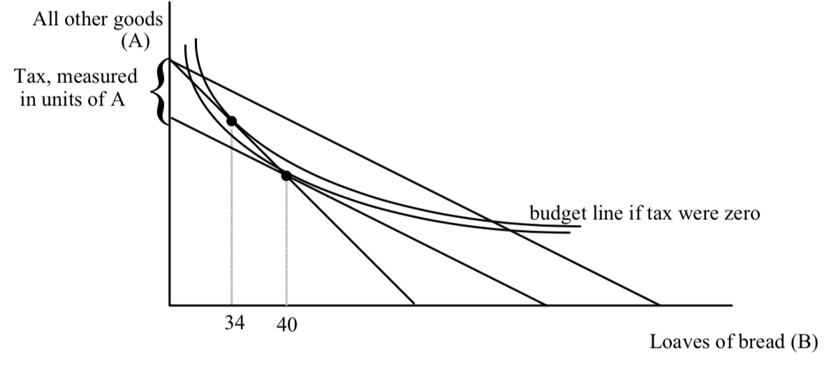
Javert originally consumes say 34 loaves, less than what will turn out to be the average under the program. He is told his tax bill will be $20. If he continues to consume 34 loaves, he will owe the government $3 at the end of the year. (CAN YOU SHOW WHERE THIS $3 DECREASE IS IN THE DIAGRAM?) So he cannot have the same amount of AOG if he stays at 34 loaves as he had before the program existed. His purchasing power is not constant but lower–he can’t get to his old tangency. The best he can do is where one of his indifference curves is tangent to his new flatter, lower purchasing power budget line. It turns out, the best he can do is to consume 40. As I have drawn it, this turns out to exactly equal the average amount of bread consumed under the program. Javert gets the neutral note–his subsidy check ($20) is exactly equal to his tax bill.
Javert is worse off. He consumes more bread than before which makes him happier–but when we include what Javert has to give up in taxes to finance the purchases of everyone else, he is worse off. If he tries to go back to 34 loaves of bread, he can no longer have the old quantity of AOG–this makes him even worse off compared to his original situation. But if everyone is average, they must all look like Javert. The average impact of a subsidy is negative. Some can be made better off (those who consume more than the average, but these losses are more than outweighed by the losses imposed on the losers.