Supply and Demand: An Introduction

Introduction

Two fundamental postulates of behavior underlie all of the analysis in these notes:

1. Incentives matter (more here)
2. Nothing is free (more here)

Almost everything else that follows comes from applying these two simple ideas in a market setting—a way of thinking about how buyers and sellers interact and the prices and quantities and other outcomes of their interactions.

Supply and Demand

Individual demand

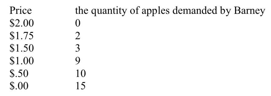
An individual’s demand curve for apples tells us how many apples a person would like to buy in a particular period of time as a function of the price. Let’s talk about Barney Rubble’s demand for apples per week. One way to represent Barney’s demand curve for apples is to use a chart. The chart shows how many apples Barney buys per week at different possible prices.

Chart 1

The information in the chart can also be captured in a graph:

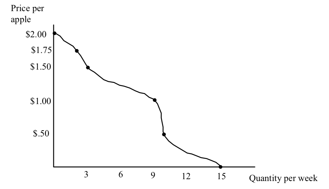
When the price of apples is $1.50, Barney buys 3 apples per week. When the price falls to $1, Barney buys more apples per week, 9. The graph tells us what Barney would do at all the different possible prices of apples. When the price of apples is more than $2, Barney finds apples too pricey and buys zero. When apples are “free”, that is when the price of apples has a zero monetary cost, Barney buys a lot, but not an infinite amount, because after a while he gets sick of apples or it takes too long to eat them and he has better things to do.¹

The demand curve is downward sloping. As apples get more expensive, Barney buys fewer. When apples get cheaper. Barney buys more of them.

The graph has an advantage over the chart; the graph shows the quantities demanded at EVERY price. The chart just shows a subset of all the possible prices. There seem to be two silly things about the graph. It assumes that there are prices such as $1.23654 per apple. But prices can be fractions of a penny in the real world. Two apples for a quarter is very close to apples selling for 12.5¢. The graph also assumes that you can buy 3.75 apples per week. The marketplace may actually allow purchases of 3.75 apples per week by selling slices of apple. Think of the market for gasoline. Alternatively, think of someone who buys 15 apples every four weeks. This is like buying 3.75 apples per week.

Barney’s quantity demanded depends on many factors other than price. We hold these other factors constant when filling in the chart or graphing Barney’s demand curve. For example, a change in information can change Barney’s demand for apples. If Barney discovers that eating apples reduces his probability of getting cancer then the numbers in the chart would change. Or suppose Barney changed jobs and in the process increased his income. At the new higher income, Barney is likely to want to purchase a different quantity of apples than he did before, AT EVERY PRICE.

A change in income is likely to change Barney’s demand for apples. A normal good is a good whose demand is positively related to income. For a normal good, the quantity demanded of apples at every price changes in the same direction as the change in income–an increase in income increases the quantity demanded at every price, a decrease in income decreases the quantity demanded at every price. An inferior good is a good whose demand is negatively related to income–an increase in income decreases demand, a decrease in income increases demand for an inferior good. These terms can be misleading because they do not have to correspond to their meanings in everyday language–an inferior good does not have to be “inferior” in the sense of second-rate, shoddy or poorly made. It may be, but it may not be.

Generic oatmeal is likely to be an inferior good for many people. As a person’s income increases, he or she buys less generic oatmeal, holding price constant. To conclude whether a good is normal or inferior, the factors other than income that affect demand must not change, or if they do, must change in a way to make a conclusion unambiguous. (If Barney’s income goes up at the same time that the price of oatmeal goes up and Barney’s consumption of generic oatmeal goes up, we can conclude that generic oatmeal is a normal good for Barney. But if Barney’s generic oatmeal consumption had gone down, we could not conclude that generic oatmeal was an inferior good for Barney. WHY?) A good can be normal for some people and inferior for others. A good can be normal at some prices, but inferior over others. Show the effect of an increase in income on the demand for apples in this case.

Another factor that could change is the price of related goods. If oranges became more expensive, Barney as a fruit-lover will buy more apples than he did before at each price. An increase in the price of oranges shifts out Barney’s demand for apples. An increase in the price of flour reduces Barney’s demand for apples if Barney likes to combine apples and flour to make an apple pie. When holding other factors constant, the price of a related good is positively related to the demand for apples, we say the two goods are substitutes. When the price of a related good is negatively related to the demand for apples, we say the goods are complements.

It is not easy to rigorously define a “related good” ex ante. In one sense, all goods are related. Consider the relationship between my demand for 100% cotton pinpoint oxford shirts and my demand for apples. They seem pretty unrelated. But suppose the price of shirts goes from $40 to $36 because of a decrease in the price of cotton. Does this affect my demand for apples? Suppose the decrease in the price of shirts induces me to buy more shirts and so many more, that my expenditure on shirts goes up. This leaves me with less income and reduces my demand for apples, doesn’t it? So aren’t apples and shirts related goods? The simple answer is that a change in the price of shirts is more likely to affect my demand for other kinds of cotton shirts than it is to affect my demand for apples and the effect on apples is probably small enough to ignore.

The Elasticity of Demand

Let’s look at the effect of the change in the price of shirts more closely. When the price of shirts goes down, I buy more shirts. What is the net effect on my expenditure on shirts? My expenditure on shirts each year is the product of the price of shirts, and the number of shirts purchased each year, PxQ. The price has gone down, and the quantity has increased. These two changes work in opposite directions on expenditure. Which effect will outweigh the other? When two numbers are multiplied together, the percentage change, positive, negative or zero, is approximately equal to the sum of the percentage changes in each component:

% change in PxQ = % change in P + % change in Q

The percentage change in P is always in the opposite direction of the percentage change in Q. (WHY?) This formula is an approximation that works well when the percentage changes in P and Q are small. Suppose when the price of shirts is $40, I buy 10 shirts a year, so PxQ is 400. If the price of shirts goes from $40 to $36 there is a 10% decrease in price, so the first term in the above equation would be -10. My quantity demanded of shirts increases. Suppose it increases to 11 shirts a year, a 10% percentage increase. So the second term in the above equation is 10. The predicted percentage change is -10+10 or zero. In fact, my total expenditure on shirts is now $396 ($36×11), almost the same expenditure, but actually a small decrease.

(There is an inherent ambiguity when defining percentage changes as to what number to use as the base for the percentage change, the starting number or the finishing one. By convention, we almost always use the starting number, so that if price falls from $40 to $36, we say there is a 10% decrease. But if price rises from $36 to $40, there is an 11% increase. If you want to avoid this ambiguity and get more accurate predictions about expenditure, you can use the midpoint between the two changes. So for example, if price falls from $40 to $36, calculate the percentage change as (40-36)/38, or a 10.53% decrease. The increase in the number of shirts from 10 to 11 is then a percentage increase of 1/10.5 or 9.52%. Because the percentage fall in price is 1.01 percentage points larger than the percentage increase in quantity, the equation predicts a 1.01% decrease in expenditure, which is very close to the actual decrease of $4.)

If, on the other hand, the 10% decrease in price had led to a larger than 10% increase, say to 12 shirts a year (a 20% increase), then the equation above says the net effect on my expenditure is the sum of a 10% decrease and a 20% increase for a net increase of 10%. Let’s see. Expenditure goes from $400 to $432 ($36×12), an increase of 8%, so the formula is pretty close. (It would do better if the percentage changes in price and quantity had been smaller. Try another numerical example yourself and see.)

If the 10% decrease in price had only increased the quantity by 5%, expenditure should fall by about 5%. A 5% increase in quantity is an increase from 10 to 10.5. (Can I buy 10.5 shirts in a year? No, but I can buy 21 shirts over two years…) Total expenditure goes from 400 to 378, a decrease of 5.5%.

Whether expenditure goes up, down, or stays the same, depends on which percentage change, price or quantity, is larger in absolute value. This in turn depends on the responsiveness of the quantity demanded to changes in price. We would like a general expression of this responsiveness of quantity demanded to price. A useful measure which captures this responsiveness is elasticity. The price elasticity of demand is defined as the percentage change in quantity for a particular percentage change in price, divided by that percentage change in price, or:

where the symbol ∆ stands for change. Because quantity always moves in the opposite direction of price, the ratio is always negative. For convenience, we will drop the negative sign, and use the absolute value of the ratio.

The price elasticity of demand must be greater than zero, because we assume demand is responsive to price, even if the effect is small. There are two important aspects of our use of elasticity as a measure of responsiveness. The first is that it does not depend on the units we measure price or quantity in. Suppose we measured price in cents instead of dollars. A 10% decrease in price from $40 to $36, is also a 10% decrease in price from 4000¢ to 3600¢. An alternative measure of responsiveness, the slope of the demand curve, would depend on the units used and thus would be unreliable.

A second important feature of elasticity is it gives us a convenient way to talk about changes in expenditure in response to price. As you might expect, the critical value for the elasticity is 1, when the ratios of change are equal, and thus just offset each other.

When the price elasticity of demand is equal to one, we say demand is unitary elastic. When the elasticity is greater than one, the quantity response exceeds the price response and we say demand is elastic. When the quantity change is smaller in percentage terms than the percentage change in price, demand is relatively unresponsive to price and we say demand is inelastic. The following chart captures some of these ideas.

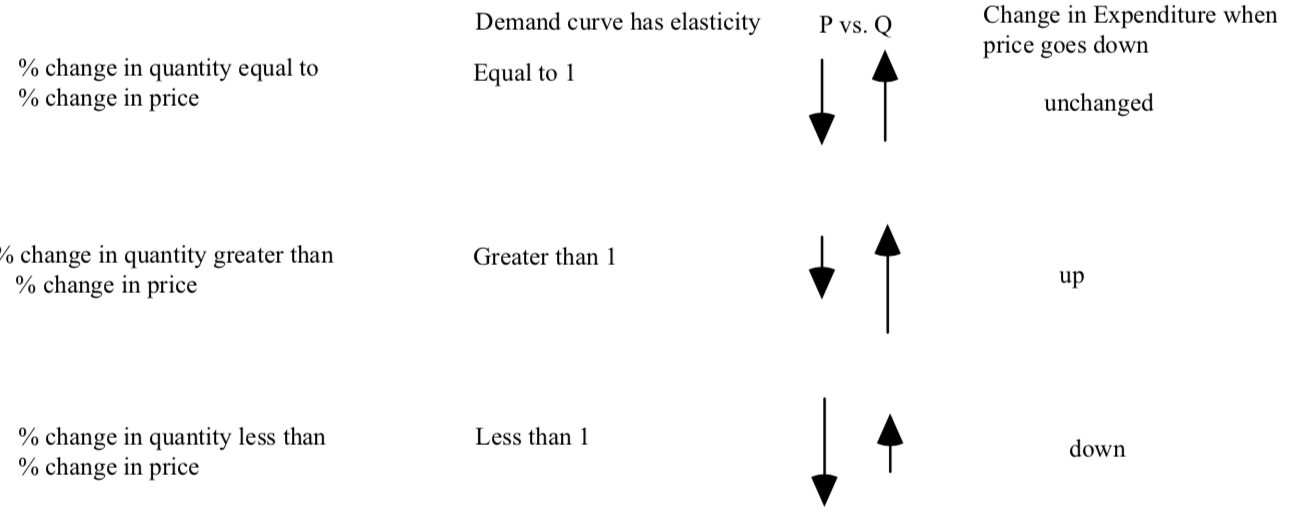The arrows in the third column are to give you an intuitive way to remember the relationship between elasticity and price. The longer the arrow, the bigger the percentage change. The arrow on the left represents a percentage change in price of a particular size. The second arrow represents the magnitude of the percentage change in quantity demanded in response to the price change. The longer the arrow, the bigger the percentage change. The longer arrow’s effect dominates the effect on expenditure except when the two arrows are the same length and expenditure is unchanged.

Now let’s use elasticity to talk about the effect of a change in the price of pin- point oxford shirts on my demand for apples. Suppose you know that my price elasticity of demand for p-p.o. shirts is equal to 4. For any percentage change in price, the percentage change in quantity will be four times larger. So if price of p-p. o. shirts falls from $40 to $36, the number of p-p. o. shirts I buy this year will go from 10 to 14. As promised in the case where demand is elastic, a decrease in price leads to an increase in expenditure. My expenditure goes from $400 to $504. What would you have predicted as the change in expenditure using the elasticity formula summing the percentage changes? How close is it to the actual change?

I have 104 fewer dollars to spend on other items. One of these items is apples. So a change in the price of p-p. o. shirts has to affect my demand for apples. Well, it does. But as you might expect, the effect is fairly small. If I am to increase my expenditure on p-p. o. shirts by $104, I will have to reduce my expenditures on ALL other items by $104. One of these may be apples, but we wouldn’t expect as large an effect on apples as we would on my cotton dress shirts that are not pin-point oxfords, and then on my non-cotton dress shirts, and then maybe on my flannel shirts. You would expect the change in my desired expenditures to affect these items much more dramatically than my demand for apples.

If we worry about this effect on the demand for apples, it is best to think of it as similar to a change in income. My apple consumption is likely to respond to a change in the price of pin-point oxford dress shirts of $4 in a very similar way as it would to an increase in my annual income of $104.

We have looked at four factors, price, information, income, and the prices of related goods, that affect my quantity demanded. Any one of the four factors will change Barney’s apple purchases. It is useful and convenient to graph quantity demanded as a function of price, holding the other factors constant. If they change, the demand curve changes. But if these factors are unchanged, the only thing changing quantity demanded is price.

There is a fifth factor we are holding constant, and that is the amount of pleasure Barney gets from eating apples relative to other activities–Barney’s tastes or preferences. If Barney suddenly likes apples more than other goods, this will increase his demand for apples. We will always assume that Barney’s tastes for apples are unchanged over time. This may not be true for all people at all times, but if it is not true we are in big trouble because economists have very little to say about how tastes change. Unfortunately, I’m not sure psychologists have much to say about it either.

What role does advertising play in changing demand? A lot of people view advertising as “making people buy stuff they don’t need.” I see it more as reminding people that a product exists. In a world of information overload advertising tries to get products up in the front of the informational queue. How does assumption affect demand analysis?

Economics says that when price goes down, quantity demanded goes up, holding tastes constant. It is true that if tastes change at the same time that prices change we don’t know what happens to quantity demanded, but then we no longer have any implications about the world and no model. So we will assume that tastes do not change. The test of the model is not whether there are times when tastes change, but whether they are infrequent enough so that the predictions we make when we assume that tastes are constant are correct.

We will allow a consumer’s information about the world to influence his or her demand. If consumers believe eating oat bran reduces the risk of cancer, the demand for oat bran will increase. This looks like a change in taste, but we will call it a change in the information set of consumers. It is a useful factor to consider because it is observable and we can often predict the direction of the effect on demand.

Suppose the price of apples is $1.50. Barney is eating 3 apples per week. Think of two possible changes that would in turn change Barney’s demand for apples. One is a decrease in the price of apples from 1.50 to 1.00. The other is a decrease in the price of oranges. The effect of the decrease in the price of apples is found by moving down the chart or moving down Barney’s demand curve from point A to point B. When the price of apples falls and Barney increases his purchases of apples we say that there is an increase in the quantity demanded.

A CHANGE IN THE PRICE OF APPLES CHANGES THE QUANTITY DEMANDED.

Barney also buys more apples when the price of oranges increases. But he will buy more apples GIVEN ANY PRICE OF APPLES. Barney’s quantity demanded when the price is $1.50 will increase, and it will increase at every price. Barney will have some new chart and new demand curve when the price of oranges falls. We call the increase in quantity demanded at every price an increase in demand.

DO NOT CONFUSE AN INCREASE IN DEMAND WITH AN INCREASE IN QUANTITY DEMANDED. AN INCREASE IN DEMAND OCCURS WHEN THE QUANTITY DEMANDED INCREASES AT EVERY PRICE. A FALL IN PRICE INCREASES QUANTITY DEMANDED.

This brings us to the law of demand. THE LAW OF DEMAND SAYS THAT HOLDING OTHER RELEVANT FACTORS CONSTANT, THERE IS A NEGATIVE RELATIONSHIP BETWEEN PRICE AND QUANTITY DEMANDED.

Market Demand

The market demand curve is the quantity demanded by all the people in the market. It answers the question: how many apples will be purchased by everyone at various prices of apples in the market. To find the market quantity demanded at a particular price, you add up all the individual quantities demanded. For example, if everyone in Bedrock were just like Barney and the population of Bedrock is 1000, then when the price of apples is $1.50, the quantity demanded by the market will be 3000 per week. The quantity demanded when the price is $1 will be 9000.

The market demand curve is found by adding up all the individual demand curves in a horizontal direction. Chart 2 shows the demand for apples by Barney, and Betty. Figure 108.12 shows the individual demand curves as dBe, dBa, along with the market demand curve for apples as if the Flinstones and the the entire market for apples in Bedrock.

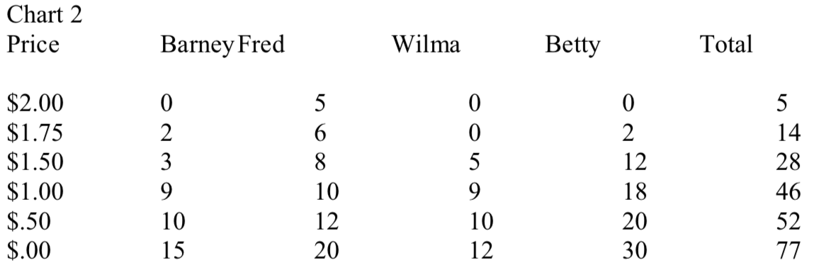
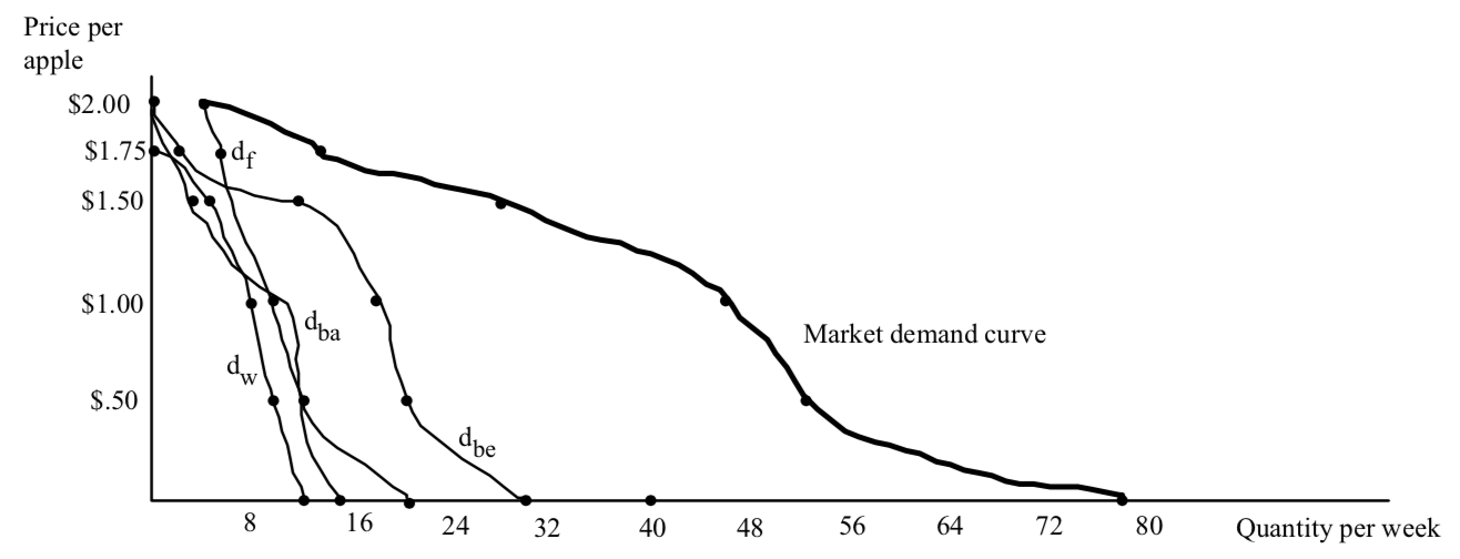
The only restriction on individual demand curves is that they slope downwards. As a result, the market demand curve, shown in bold, also slopes downward. The market demand curve is the horizontal sum of the individual demand curves. It is the horizontal sum in the sense that at each price, you take the horizontal distance on each individual demand curve, add these numbers up, and you get the point on the market demand curve at that price.

Supply

The firm’s supply curve is the quantity supplied by the firm at various prices. Suppose there are many different firms in Bedrock who grow and sell apples. Let’s look at one of them, the Jetson Apple Farm. The chart shows the quantity supplied of apples at various prices by the JAF:

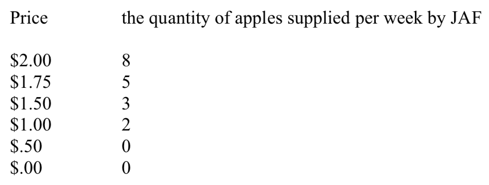
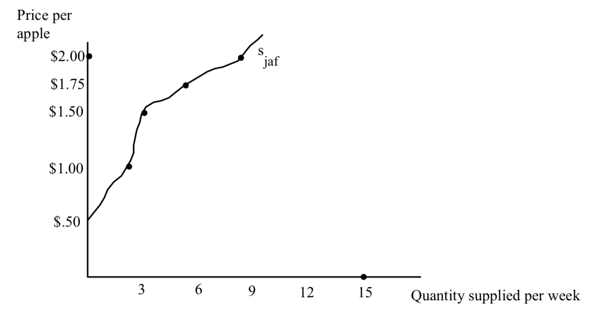
There are two interesting things about the chart. As price increases, JAF is willing to supply more apples to the market. The other interesting part of the chart is that there is a minimum price before JAF is willing to sell any apples. From the chart we know that the minimum price is something between $.50 and $1.00, but we can’t tell exactly unless we filled in some more entries in the chart. Just as in the case of demand, we can represent the firm’s willingness to supply apples with a supply curve, showing the quantity supplied by the firm at every price:

A FIRM’S SUPPLY CURVE IS THE QUANTITY OF APPLES SUPPLIED AT VARIOUS PRICES PER UNIT OF TIME.

Suppose price is $1. At a price of $1, the firm would like to grow and sell two apples per week. What could cause the firm to want to grow and sell more apples than 2 per week? One answer we already know: an increase in the price of apples will make the firm want to supply more apples. We see that in the chart as a move from one cell in the chart to another cell. We see it in the graph as a movement along the supply curve.
AN INCREASE IN PRICE INCREASES THE QUANTITY SUPPLIED. A DECREASE IN PRICE DECREASES THE QUANTITY SUPPLIED.

Just as in the case of demand, we make a distinction between a change in the quantity supplied and a change in supply. A change in quantity supplied occurs when there is a change in the price. A change in supply is when there is a change in something other than price that causes the firm to change its quantity supplied AT EVERY PRICE. Factors that change the SUPPLY CURVE include:

1. The wage of laborers used to grow and pick apples
2. The price of machines used to grow and pick apples
3. The price of apple seed
4. The cost of the land
5. The technology of apple production.

The first four are called changes in INPUT prices. An input is anything the firm has to pay for either by renting or buying in order to produce additional apples. When an input becomes more expensive, for example, the firm will find it profitable to produce and sell fewer apples at every price. There is a decrease in the firm’s supply curve. When input prices fall (so that it becomes cheaper to produce apples) firms will wish to sell more apples at every price. The supply increases.

Notice that I did not list the price of the land but rather the cost of the land. What is the cost of the land? The cost of any item is not necessarily what you pay for it but what you have to give up to have it. These may be the same thing. The cost of an apple to me, Russell Roberts, apple eater, is the money it takes to buy an apple in the grocery. But even this is not exactly right. The money I have to pay for an apple is the cost of acquiring an apple, but it is not the cost of eating an apple. The cost of eating an apple is the money I have to pay, plus the value of the time it takes to eat it, plus the reduced room in my stomach for other foods. Those are the things I give up in order to eat an apple.

The true cost of an item includes everything I give up to use the item in a particular way. The cost of attending college is not merely the tuition, but the wages you cannot earn because you cannot earn money as effectively while you are going to college. The cost of using land to grow apples is not just what I paid for the land, but the value of using the land for the best alternative use other than apples. If I can grow pears on the land and the price of pears goes up, it becomes more expensive to grow apples given any price of apples, and the supply of apples will decrease, shifting in and to the left.

If I am the owner of a firm I have to decide whether to buy or rent my equipment. Suppose I decide to buy. If, for example, I own my own trucks for example for delivering my product, and the price of RENTAL trucks goes up, does this affect my supply curve? After all, if I own my trucks, are rental trucks one of my inputs. Indirectly, yes. As a truck owner, the price of rental trucks is part of opportunity cost. The cost of owning trucks is the fact that I could rent them out. When the price of rental trucks goes up it is more expensive to own trucks. I may choose to rent out some of my trucks I used to use for delivery.

The fifth item, technology, is the knowledge a firm has about how to combine the inputs to produce apples. If a firm learns a new way to combine inputs and get more apples than before from the same amount of inputs, we say there is a technological advance, and the firm will wish to sell more apples at every price compared to before. So technological advances increase supply, shifting the supply curve down and out. Any time we draw a supply curve for a particular firm, we are holding constant input prices and technology. A change in any of these factors will shift the entire supply curve. A change in price is a movement along the supply curve. DO NOT CONFUSE A CHANGE IN SUPPLY WITH A CHANGE IN THE QUANTITY SUPPLIED. A CHANGE IN SUPPLY IS A SHIFT OF THE ENTIRE CURVE. A CHANGE IN THE QUANTITY SUPPLIED IS A MOVEMENT ALONG THE CURVE DUE TO A CHANGE IN THE PRICE OF THE ITEM BEING SUPPLIED.

The market supply curve is the quantity supplied by all the firms in the market at
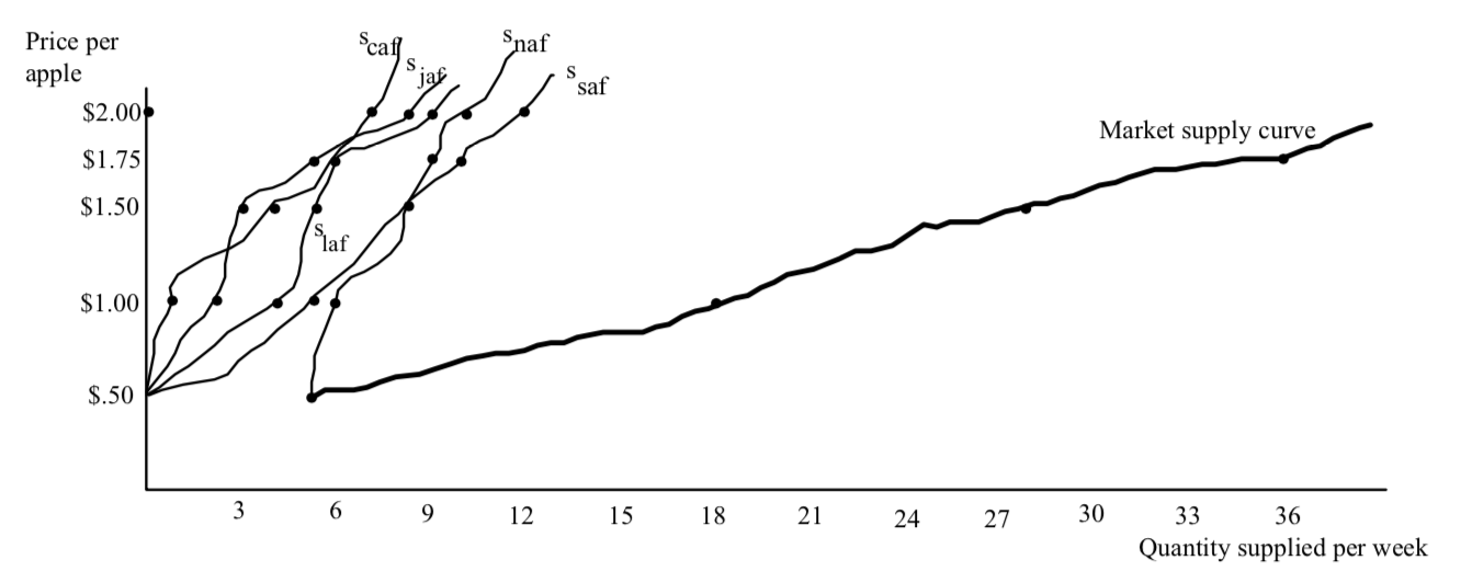
various prices. Suppose the Jetsons are just one of many apple farms in bedrock. There is also the Luke Apple Farm, the Solo Apple Farm, the Clarence Apple Farm, and the Nimoy Apple Farm. The following chart shows the quantity supplied by each firm at various prices:

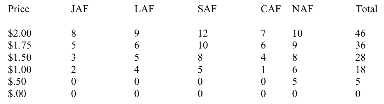Notice that for each firm, there is an increasing relationship between price and quantity supplied. As a result, the market quantity supplied is increasing in price, guaranteeing that the market supply curve is upward sloping with respect to price. (WHY MIGHT EACH FIRM HAVE A DIFFERENT SUPPLY CURVE AS I HAVE ASSUMED IN THE CHART?) As in the case of demand, the market supply curve has more information that the above chart because it shows the quantity supplied by all the firms at all prices, not just the prices shown in the chart. This is shown below:

Suppliers and demanders make up the two sides of the market. The demand curve tells us how demanders respond to price holding tastes, income, and the prices of other goods constant. The supply curve tells us how suppliers respond to price holding input prices and technology constant. The demand curve tells us how demanders respond to price holding tastes, income, and the prices of other goods constant.

We can use supply and demand to determine what will be the price of apples:

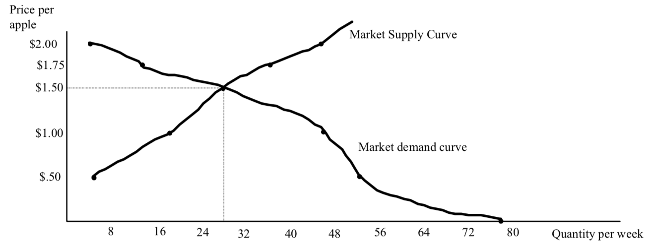There is a single price where, P*, where quantity supplied equals quantity demanded. There is something very special about the price where quantity supplied is equal to quantity demanded. In our case, this price, P* is $1.50. When price is $1.50, quantity supplied equals quantity demanded.

At any other price quantity supplied does not equal quantity demanded. Suppose all suppliers post a price of $2.00 per apple each week. Can this situation persist? It is unlikely. At a price of $2.00, suppliers in the aggregate would like to sell 46 apples. But consumers will only wish to buy 5 apples. Sellers will find that 41 of their apples go unsold. THERE IS EXCESS SUPPLY. (We don’t know where these 41 apples will be in the sense that we don’t know which suppliers will have which share of the 41 apples. All we know is that 41 apples will go unsold.) The suppliers with unsold apples will lower their price in order to get rid of their unsold apples. Price will start to fall throughout Bedrock. What is the force that causes price to fall–competition among sellers to get rid of their apples.

Next week fewer apples will be brought to Bedrock and they will be sold at a lower price. Suppose suppliers show up and post a price of $1? At a price of $1, the various suppliers bring 18 apples to their stores, while consumers in the aggregate will try to purchase 46 apples. There is EXCESS DEMAND. Consumers will find that there are not enough apples to go around at a price of $1. Suppliers will find themselves running out of apples in the middle of the day and that consumers continue to show up wanting to buy apples. As suppliers run out of apples to sell, they will start to raise the price as consumers compete to get at the increasingly scarce supply of apples. When there is excess demand, competition among demanders drives up price. Suppliers will realize that they could have sold more apples at a higher price. Next week they will bring more apples to the market and charge a higher price.

There is only one price, $1.50, where suppliers and demanders have no incentive to drive price either up or down. The price where quantity supplied equals quantity demanded is the equilibrium price. The equilibrium price is the price that persists unless something changes. In our case, the thing that might change might be income of consumers or technology or any of the other factors held constant along either the supply or demand curve. There is one other very important factor that might change and that is the rules of the game–how suppliers and demanders are allowed to interact. Right now we are assuming that suppliers and demanders are free to bargain over price. Soon we will consider cases where the government places restrictions on the prices sellers can charge and buyers can pay.

Now suppose there is an increase in demand. Price rises to $2.15 and the quantity bought and sold increases to 40. Why did the price increase? At the old price of $1.50, given the new demand curve, there is now excess demand. (Can you see it in the graph– where is it?) Competition among buyers will drive up the price until the new price of $2.15 is reached. Given the new demand curve, there is only one price where quantity supplied is equal to quantity demanded.

Suppose you look at the real world and you notice that the price of apples has gone up from $1.50 to $2.15, and the quantity of apples purchased has also gone up, from 28 to 46. You might be tempted to say something like this: “You have told me that demand slopes downward. But I have just seen a situation where price went up and people bought more apples. This refutes the law of demand and means that economics is worthless.”

STOP READING. WRITE A ONE PARAGRAPH RESPONSE TO THIS STATEMENT. IF YOU DON’T KNOW WHERE TO START, GO BACK TO THE DEFINITION OF THE LAW OF DEMAND.

The mistake is to confuse the demand curve with the quantity demanded. An increase in demand increases price. This leads to a new equilibrium where the quantity bought and sold has gone up. The law of demand still holds–if the factors held constant along the demand curve stayed constant and price went up (IF THE FACTORS HELD CONSTANT ALONG THE DEMAND CURVE WERE TO STAY CONSTANT, WHAT MIGHT CAUSE PRICE TO RISE?), then quantity demanded would fall just like the law of demand says it would.

In fact, we implicitly used the law of demand to get to the new equilibrium. One way to think about how the new equilibrium is achieved is to think of price staying at $1.50 given the new demand curve. There is excess demand. This puts upward pressure on price as demanders compete to get at the scarce apples. As price rises, two things are happening to cause quantity supplied to equal quantity demanded. Quantity demanded is falling, we are sliding up the new demand curve, and quantity supplied is increasing as we slide up the old supply curve. Eventually we get to a new equilibrium where quantity supplied is equal to quantity demanded.

This last story is a story of how the market moves from one equilibrium to another. It is just a story. Economists do not know a great deal about the precise path between two equilibria and how long it will take. WE WILL ASSUME IN HERE THAT SUCH ADJUSTMENTS ARE INSTANTANEOUS AND THAT MARKETS ARE ALWAYS IN EQUILIBRIUM. THAT IS, WE WILL ASSUME THAT PRICES ADJUST TO EQUATE QUANTITY SUPPLIED WITH QUANTITY DEMANDED. If you can remember and learn to apply that last phrase in bold face you will go a long way towards being an economist. Unfortunately, it is not so easy.

Here is a problem to see if you understand equilibrium and how to use supply and demand. Suppose people with heart disease in their family are told that eggs are bad for their cholesterol level and that they should stop eating eggs. Suppose people with heart disease believe this to be true and that cholesterol is only relevant for people with heart disease in their family.

1. What happens to the price of eggs?
2. What happens to the consumption of eggs by people without heart disease in their family?
3. What happens to the total number of eggs bought and sold?

To summarize:

In an unconstrained market, that is, in a market where consumers and producers are free to make bargains with each other without restrictions on price, the equilibrium price is where the market supply curve crosses the market demand curve. We call this price P*, and the quantity where the two curves cross is Q*. Given the market price of P*, we can go back to the individual supply and demand curves to determine the consumption of each individual consumer and the production of each firm.

Four Common Mistakes People Make When Using Supply and Demand

It’s easy to see that supply and demand usually cross somewhere and to call where they cross on the vertical axis P* and where they cross on the horizontal axis Q*. Not surprisingly, it is a lot harder to use supply and demand as in the egg problem above. Here are some common mistakes people make when using supply and demand.

Mistake #1–Confusing movements along a curve with a shift in the curve

Suppose the income of consumers decreases and apples are a normal good. What happens to the price of apples? Here is a flawed chain of logic: “If income goes down and apples are a normal good, the demand for apples decreases. When the demand for apples decreases, the price of apples goes down. When the price of apples falls, demand increases pushing price back up. So the net effect on the price of apples is uncertain.” The speaker confuses a shift in demand with a movement along a demand curve. The decrease in income does reduce the demand for apples. The decrease in the demand for apples does reduce the price. But the reduction in price does not increase demand. It increases the quantity demanded–a movement along the curve. At the original price, there is excess supply when demand decreases. Price must fall to eliminate this excess supply. The excess supply is eliminated by the decrease in price–as price falls, quantity supplied decreases, and quantity demanded (along the new demand curve) increases. At the new equilibrium, there are fewer apples bought and sold and the transactions occur at a lower price.

Remember: changes in price don’t shift the demand curve–they are movements along the demand curve.

Mistake #2: When something changes to shift the supply curve, you shift the demand curve.

Suppose the price of artificial sweetener goes up. What is the affect on the quantity bought and sold of diet soda? Here is a flawed chain of logic: “When the price of sweetener goes up, supply decreases because the price of an input has increased. This by itself would increase price. But when people see the price of the sweetener go up, they decrease their demand for soda, lowering price. The net effect on the price of diet soda is ambiguous.” This is just a roundabout way of making the same mistake made above but in a more complicated manner. The speaker could have said: “When the price of soda goes up due to the decrease in supply, this price increase decreases demand and lowers the price of soda.” When I write this way, it is easier to see how the speaker is confusing a movement along the curve with a shift in the curve. The increase in price decreases quantity demanded, it doesn’t decrease demand. The supply curve shifts in and to the left, the equilibrium price rises to close the excess demand at the old price; this increase in price reduces quantity demanded, increases quantity supplied; at the new equilibrium price is higher, and quantity bought and sold is lower.

But let’s give the speaker a chance to defend himself: “Look,” he says belligerently, “are you trying to tell me that when the price of sweetener goes up people aren’t going to buy fewer sodas? And isn’t that a decrease in demand?” When the price of sweetener goes up, ultimately people are going to buy fewer sodas. But this is not a decrease in demand. This is due to an increase in the price of soda caused by a decrease in supply caused by that increase in the price of sweetener.

The easiest way to see the flaw in the more sophisticated argument of the speaker is to think of making a trip to the soda machine when sodas are 50¢, before the increase in the price of the sweetener. At the price of 50¢ you buy some number of sodas per week, say 9. Now suppose you read in the paper that the price of sweetener has gone up. IF when you return to the machine the price is still 50¢, are you going to behave any differently? You are still going to buy 9 sodas per week. (I’m assuming you can’t store sodas. If you could, the answer is more complicated and more interesting, but we’ll delay that analysis for a bit.) You’re not going to say, “Well, soda is more expensive because sweetener is more expensive, I’ll buy less soda.” What will instead happen is that when you arrive at the soda machine sometime after the sweetener price increase, you will see the price is now 60¢, say, and you will purchase fewer sodas. But this is a movement ALONG your demand curve–a change in your quantity demanded in response to a change in price.

Mistake #3–Confusing a Change in the Equilibrium Quantity with a Shift in Supply or Demand

Once again this mistake is avoided if you keep straight the difference between a shift in the curve and a movement along the curve. Suppose you observe a housing boom in a city. What does supply and demand have to predict about what will happen to price? A common mistake is to say: “If there are more houses, the increase in supply should lower the price of houses.” But an increase in the number of houses is not an increase in supply. An increase in supply is when at every price of housing, builders want to build more houses. An increase in supply could be caused by a decrease in the price of lumber. But observing more houses being built could be due to something else. Suppose a number of new companies have relocated in the city causing an increase in employment and an increase in demand for housing. An increase in demand will also increase the equilibrium number of houses. But houses will be more expensive. The bottom line: an increase in the observed quantity of a good tells you that either demand or supply has shifted. But price could fall or rise depending on whether demand or supply has increased.

Mistake #4–Confusing What People Are Willing To Pay With What They Have To Pay and Confusing What Firms Would Like to Charge With What They Have to Charge

This is also a subtle variation on some of the above mistakes. Let’s take two examples in the gasoline market to illustrate this mistake. Suppose Exxon has an oil spill. Very little oil is lost but there is massive environmental damage. Exxon incurs large costs of cleanup and compensation to fishermen. What happens to the price of Exxon gasoline? The bad economist speaks: “Exxon gasoline has to get more expensive. Exxon will raise its prices to cover the cost of the oil spill. Consumers are willing to pay more because they realize Exxon’s costs have gone up.”

The speaker makes two serious mistakes here. Exxon wants to charge more to cover its costs of the oil spill, but it always wants to charge more–it doesn’t take an oil spill to bring out Exxon’s desire for higher prices. What stops Exxon from charging more without an oil spill? Competition. If Exxon charges more for gasoline it loses customers to other brands. The same force of competition stops Exxon from raising its price when there IS an oil spill. Perhaps Exxon’s desire for higher prices is more intense after its costs have risen, but it will be just as impotent as before in carrying out this desire.

“But,” says the speaker, “people will be willing to pay higher prices if Exxon has higher costs.” Oh really? They are willing to pay more in a sense–if the price of gasoline goes up, most people ARE willing to keep buying SOME gasoline, though they will buy less. But just because they are willing to pay more, they don’t have to. They will turn to other brands. Imagine going to buy a pair of shoes at your local mall. You go to the store you usually go to and find that the prices seem awfully high. Asking a salesman about the prices, he shrugs and says, “Yeah, sorry about that. But the boss’s daughter was married last month and he’s kind of strapped for cash. So you’ll understand why he’s increased all prices by 30%. And you won’t mind paying a higher price will you?” Are you willing to pay a higher price? You might be, even if you’ve never met the daughter and missed the wedding. It’s possible you might still get positive consumer surplus from purchasing the shoes even though the price is 30% higher. But your consumer surplus is even higher if you go next door and buy the shoes from a different store in the mall at a lower price. You’re willing to pay more, but you don’t have to.

A more sophisticated version of this mistake occurs when considering the effect of a large oil spill that significantly affects the total amount of crude oil available for refining. A decrease in the amount of crude oil means a decrease in the quantity of gasoline in the future when the crude oil would have been refined. But there is no less gasoline now simply because there is less crude oil now. Oil companies would like to increase their prices, using the oil spill as an “excuse.” Are consumers willing to pay more because of the spill? By itself, the spill has no effect on consumer’s willingness to pay for gasoline. Consumers are willing to pay more for gasoline, but they are always willing to pay more for gasoline. IF the price of gasoline rises, people will buy less gasoline. If the price of gasoline rises, oil companies will want to supply more gasoline. Unless something shifts the supply or demand curve, the desire of gasoline companies to increase their prices is not going to make prices go up. If prices do go up, there will be excess supply and price will come back down. To see this more dramatically, suppose oil companies showed a video of an enormous oil spill. Does this shift out consumers’ demand curves and allow a higher equilibrium price of gasoline? NO.

Storable Goods

Because gasoline can be stored, an oil spill today CAN affect the price of gasoline today. When a good can be stored, the price tomorrow can affect the supply curve today. If the price of gasoline is expected to be higher tomorrow than it is today, then profits can be made by buying gasoline today at a low price today and storing it, and selling it tomorrow when the price is higher. An oil spill today, if it is large enough, can create an expectation that the supply will be lower tomorrow, so price of gasoline is expected to be higher tomorrow. This expectation of a higher price tomorrow means profits can be made by storing gasoline. The amount supplied this period goes down, and price goes up. TRY AND DRAW A GRAPH TO CAPTURE THIS STORY. You can actually show that the act of storage of gasoline is beneficial to society. Speculators, people who buy commodities now hoping that their price is going to rise, provide an important service to society–they smooth out shortages so the path of prices is smoother than it would otherwise be. We could show how this produces a net gain.

Now let’s try this same story with the video of the spill. If suppliers show the video, they can only raise prices if there is less gasoline available today. There would be less gasoline if suppliers responded to the video by storing gasoline. But if they store gasoline today hoping to sell it for a higher price tomorrow, then they will find out they are wrong. Unless there is an actual spill, there is no profit to be made from storage. What role does the video play in this story? (None at all–it just shows the fallaciousness of thinking that consumers will pay a higher price and keep buying the same quantity if they think the higher price is “justified.” Of course producers could all get together anyway and withhold supply today even without the video. What makes this hard to do?

The Magic of Prices

Prices adjust to equate quantity supplied and quantity demanded. It is that equilibrating role of prices that lets firms use the market to provide inputs to production rather than being vertically integrated. The equilibrating role of prices gives firms confidence that they can always find inputs available so that a pencil manufacturer don’t have to own a graphite mine to insure supply. That allows them to avoid having to acquire the knowledge you need to run a graphite mine, run an aluminum mine and aluminum smelter, a cedar farm, etc and lets people specialize.

When we think of specialization, we think of “practice makes perfect.” But practice also make boring. The hidden power of specialization isn’t just that power of getting better at something simply by doing one thing over and over. The real power comes from having the right people in the right jobs. It comes from WHAT you specialize in as much as anything else.

One downside of relying on markets is that you are then subject to price fluctuations. But the market solves this problem in a variety of ways. Can you think of any?

So prices eliminate shortages and allow the power of specialization to be unleashed. That in turn allows knowledge to be spread out via specialization. How does it get pooled back together?

There are two senses in which the knowledge gets pooled. Take a pencil. All that knowledge of all the different materials. How does it get successfully coordinated? And how does it get successfully coordinated for only 25¢? Prices again play the key role here, combined with the voluntary interactions of buyers and sellers. When I’m a pencil manufacturer I don’t need to research whether the aluminum seller has the right mix of workers and techniques. I just look at the price and the quality of the service. Price competition (a fancy way of saying that I’m free to shop around and look for the best deal) induces suppliers to minimize their costs and find the most effective way of providing the good. (I almost said the best way. Why did I change that word?) So prices don’t just insure that supply is available. They provide the incentive for suppliers to please their customers.

Finally, prices have at least one more role to play. When the situation changes, when the demand for graphite increases because there’s an increase in the demand for cars, not only do prices insure that everyone who wants to pay a premium can still get graphite, it tells all of the demanders of graphite to find ways to economize on graphite. Here, prices perform the role of both signal and incentive. The higher price tells people to cut back or find alternatives and it gives them an incentive to find those alternatives. That in turn creates the incentive to create the knowledge we talked about last night, the knowledge of how to cope with the reduced availability.

As beautiful and remarkable as all of this is, there are two more remarkable things to note. First, price doesn’t just go up when graphite demand goes up. It goes up by the right amount necessary to induce the changes we’re talking about. Not too much and not too little. (Is this true in the real world or just in our instantaneously adjusting models?)

The last most remarkable thing of all is that prices emerge. No one is charge of them. They emerge out of the buying and selling. There isn’t a market for graphite, really. “A market for graphite” is an intellectual construct to help us talk about this incredible phenomenon the orderliness of the prices that emerge and the behavior they engender, the knowledge they create and coordinate.

For an exploration using supply and demand to understand the role of prices in creating information and putting it to use, see my essay “How Markets Use Knowledge.” For a less formal look at markets as a marvel, see my essay, “A Marvel of Cooperation: How Order Emerges Without a Conscious Planner.” And for additional readings and other media around emergent order, see my animated poem, “It’s a Wonderful Loaf” and go here.